We are bounded in a nutshell of Infinite space: September 2015

Monday, September 28, 2015

Aristarchus, the first Heliocentrist

We are bounded in a nutshell of Infinite space: Blog Post #13, Biography #1: Aristarchus, the first Heliocentrist

After the time of Aristotle and Plato, much of the Ancient Greek astronomical tradition was supplanted by Aristotelian principles. But in reality, many of the Ancient Greek scientists were closer to the truth than the principles Aristotle and other philosophers of his age would postulate, which would remain as the dominant ideas of the universe for centuries to come. With men like Democritus, Thales, and Anaximander, the so called Ionian scientists preserved an ideal that was closer to a modern view of the scientific method than that which the Athenian philosophers maintained. However, with the third century BCE more and more individuals arose that followed a more scientific approach to the description of the physical world.

One such man is Aristarchus of Samos, the first known proponent of the heliocentric model of the solar system and the one who calculated the sizes of the Moon and Sun to a degree of accuracy remarkable for his lack of precise instruments. He lived from 310 BCE to 230 BCE, working in Samos and publishing several works, of which only one has directly survived, On the Sizes and Distances of the Sun and the Moon, which shows his estimates and measurements of the Sun and Moon, as inaccurate as they may be. Here, he used not much other than his sight to estimate angles and use geometry to reach an approximation of the sizes of these objects in comparison with the Earth. Some of these estimates are rather close to actual values, while others are completely disparate from the known values (such as the sun being 20 times larger than the Earth, when it is actually 400 times larger).

Nevertheless, Aristarchus is referenced in Archimedean books which relate how he was among the first to ever postulate that the Earth orbits the Sun, as well as the hypothesis that the universe is much more than just a solar system, rather it stretches out to where there are stars (like the sun) farther away and others are nearer. His theory, overall, was the understanding that the universe stretched out into the heavens, and he also thought that distant stars had a parallax, but too small to be seen with the instruments of his time.

In all, Aristarchus was among the first to truly begin to wonder about the greater scheme of the universe. He was among the first to question the geocentric model and begin to see a simpler view of the movements of heavenly bodies.

Reference: http://www.britannica.com/biography/Aristarchus-of-Samos

Photos taken from: https://upload.wikimedia.org/wikipedia/commons/2/2b/Aristarchus_working.jpg & https://upload.wikimedia.org/wikipedia/commons/9/98/Aristarchos_von_Samos_%28Denkmal%29.jpeg

Relativity, yes we are doing this, it is what it is, it’s not as bad as it seems.

We are bounded in a nutshell of Infinite space: Blog Post #12, Free Form #2: Relativity, yes we are doing this, it is what it is, it’s not as bad as it seems.

On one of the most recent entries, we went over the nature of relativity and the role it plays when analyzing microlensing and other astrophysical phenomena that have to do with light and gravity. But what exactly is relativity, the mythical and wonderful description of the universe compiled, proved, and understood first by Albert Einstein in the first decade of the twentieth century?

As we had presented in an earlier blog post:

“Relativity describes the nature of the Four-dimensional world we inhabit, these dimensions being length, width, height, and time, 3 space dimensions and a time dimensions. Working off this knowledge, Einstein developed a description of all space as truly being a sort of fabric, a space-time fabric, whose perception is changed based on individual reference frames (from where you observe the event(s) ). Adding in the nature of the speed of light in a vacuum, the one absolute constant in the universe, and the nature of gravity and how it warps space time, bending the fabric, we can understand how light is affected by gravity.”

Thus, we have briefly explained the effect of gravity and light when these two interact with one another, but we have not delved into the inner nature of relativity, and the most important realization that serves to understand the what is actually occurring not only when gravity is in play, but in all physical reality.

The understanding that cements all relativity, and re-defined physics, was establishing that there is one universal constant in the universe, one fact that never changes, from which all of relativity is derived: the speed of light is the maximum speed of the universe, an unchangeable value that will always be the same while in a vacuum (light can change speed and direction when it changes the medium it goes through). Why is light constant?, you might ask: because it needs to be, and the evidence that proves it is more than conclusive. But another explanation for why it is constant is that light (and by this we mean the entire electromagnetic spectrum) is one of the 4 fundamental forces of nature, and thus mold much of reality around themselves.

Regardless, the fact is that light is assumed to be constant in any case, and because of this, many sets of equations were created, none of which have been dis-proven after many tests and experiments, essentially confirming that relativity with a constant speed of light is the most plausible system.

Now then, as to the actual effect light has on objects and reference frames, this is when things get a bit more confusing. So light we have just seen that it has to be constant in any circumstance, so all other variables, like space and time, are the ones that must change and make accommodations in order to maintain a constant speed of light. The classic example Einstein gives in his papers on Special and General Relativity is the case of two persons, one on a train heading in a direction towards a point where a lightning bolt just hit the ground, and another person stands some distance away and can observe both the train and the lightning bolt. In this scenario, the person on the train is moving at a speed v, who will hit the rays of light with this speed and thus (one would expect to) perceive the speed of photons as the intrinsic speed of light minus the speed of the person. This would differ from the person outside the train, seeing the lightning bolt come and thus (expect) to perceive light at its normal speed.

However, the speed of light must be CONSTANT at all times, so the person on the train must have something change in order for him to experience the speed of light at the correct value. What happens is, as Einstein describes in Special Relativity, that the person moving with speed v experiences time (and length and differently, it slows down in his (moving) reference frame and so the speed of light he perceives is maintained at the constant rate.

For the person outside the train, he would see the light coming from the lightning bolt at its normal speed, without any special considerations to be taken into account. But as he sees the light going towards the train in the distance, he would clearly see the light in direction of the train has the same speed as the light that reached his reference frame, maintaining the constant speed of light and set consolidated with the perception of the person on the train, instead of two people experiencing two different speeds of light.

This sums up the overall principles of relativity, but additionally gravity comes into play in a deeper sense and with it the entanglement of quantum mechanics and how it can (or cannot) be consolidated with general relativity, which we will leave for another time.

Nevertheless, this sums up a lot of the intuitive nature of relativity, and hopefully compels you to believe the speed of light never changes, but of you are not, go and prove it (just bear in mind people have been trying to do just that for about a century).

What does microlensing look like?

We are bounded in a nutshell of Infinite space: Blog Post #11, Worksheet # 4.1, Problem #3: What does microlensing look like?

3. When speaking about microlensing, it is often easier to refer to angular quantities in units of \(\theta_E \). Let’s define \( u \equiv \beta/\theta_E\) and \(y \equiv \theta/\theta_E\).

(a) Show that the lens equation can be written as: \[ u = y - y^{-1} \]

(b) Solve for the roots of \(y(u)\) in terms of \(u\). These equations prescribe the angular position of the images as a function of the (mis)alignment between the source and lens. For the situation given in Question 2(f) and a lens-source angular separation of 100 \(\mu as\) (micro-arcseconds), indicate the positions of the images in a drawing.

(a) From previous problem, the equation for a lens is given as \[\beta = \theta - \alpha^{\prime} , \] establishing how the differences in angle between the image seen, the original source, and the lens can be equated, seen in the following illustration:

In another problem, \(\alpha^\prime \) was also expanded on, taking into consideration the actual relativistic effects of lensing (using 4 instead of 2 in the \(\delta v\) equation). The equation for \(\alpha^\prime \) is : \[\alpha^\prime = \frac {4 G M_L}{\theta c^2} (\frac{D_S - D_L }{D_S D_L}) ,\] where \(D_S \) and \(D_L\) are distances between the Source the observer and the distance between the Lens and the observer. This equation is worked off the equation seen in the previous problem solved for angle \(\alpha\) and the expanded lens equation given: \[\beta = \theta - \alpha^\prime , \] \[\beta = \theta - (\frac{D_S - D_L }{D_S D_L})\alpha , \] \[\beta = \theta - \frac {4 G M_L}{\theta c^2}(\frac{D_S - D_L }{D_S D_L}). \] Now notice how all these equations are closely tied to \( u = y - y^{-1} \) with the definitions for u and y given at the start of the problem. Now let us divide all by \(\theta_E\): \[\frac{\beta}{\theta_E} = \frac{\theta - (\frac{D_S -D_L }{D_S D_L})\frac {4 G M_L}{\theta c^2} }{\theta_E} , \] and now we have: \[ u = y - \frac{(\frac{D_S - D_L }{D_S D_L})\frac {4 G M_L}{\theta c^2} }{\theta_E} . \] And \(\theta_E\) is actually defined by factoring out the \(\theta\) in the lens equation when \(\beta \) is 0, (\(\theta_E \) is the Einstein ring radius, a circle which forms around the Lens when the Source is directly behind it), which turns into: \[\theta_E = \left(\frac {4 G M_L}{ c^2} (\frac{D_S - D_L }{D_S D_L})\right)^{\frac{1}{2}} .\] When we substitute this into the new lens equation with u and y we have: \[ u = y - \frac{(\frac{D_S - D_L }{D_S D_L})\frac {4 G M_L}{\theta c^2} }{\left(\frac {4 G M_L}{ c^2} (\frac{D_S - D_L }{D_S D_L})\right)^{\frac{1}{2}}} , \] and many things start to cancel out after \(\theta \) is taken out as a factor of the denominator:

\[ u = y-\frac{\left(\frac {4 G M_L}{ c^2} (\frac{D_S - D_L }{D_S D_L})\right)^{\frac{1}{2}}} {\theta} , \] which, in effect is the inverse of y, \(\frac{\theta_E}{\theta} . \)

(b) This part of the problem asks us to solve for \(y(u)\), which means the new lens equation must be re written again. We take the original equation: \[ u = y-y^{-1} , \] and multiply all values by y to yield: \[ yu = y^2 - 1 ,\] \[ 0 = y^2 - yu - 1 ,\] and we solve for y using the quadratic formula: \[ y(u) = \frac{u \pm \sqrt{u^2 + 4}}{2} .\] Next we use understand the values from a previous problem referenced in the question. So the lens angular separation is: \[\beta = 100 \mu as = 1\times 10^{-1} miliarcseconds , \] and the Einstein ring radius is: \[5.6 \times 10^{-1} mili-arcseconds . \] The Einstein ring radius is found by plugging in \(M_L = 0.3 M_\odot , \) \(D_L = 4kpc , \) and \(D_S = 8kpc \) into the \[\theta_E equation \to \left(\frac {4 G M_L}{ c^2} (\frac{D_S-D_L }{D_S D_L})\right)^{\frac{1}{2}} . \] Now then, by dividing \(\beta\) and \(\theta_E\) values, we now have the value of u, which is \(\approx 1.8 \times 10^1 \), a unit-less value that serves to find what proportion to the Einstein radii the image is found. This value is now plugged into: \[ y(u) = \frac{u \pm \sqrt{u^2 + 4}}{2} ,\] and yields two values: \[ y(1.8 \times 10^1) = 9 \times 10^{-2} \pm 1 ,\] depending on whether the 1 is positive or negative.

The two values, 1.09 and -0.91, are the percentages of the Einstein radii where the image is found, as 0.18, the value of u, is the percentage of the radii where the original source is. This can be viewed as:

Where \(I_1\) is the 1.09 value image, \(I_2 \) is the -0.91 value image, L is the lens, and S is the original source.

What happens when the photons are there but the star is not

We are bounded in a nutshell of Infinite space: Blog Post #10, Worksheet # 4.1, Problem #1: What happens when the photons are there but the star is not

1. Mass bends space-time! This is a prediction of general relativity, but fortunately we can heuristically derive the effect (up to a factor of 2) using Newtonian mechanics and some simplifying assumptions.

Consider a photon of “mass” \(m_\gamma\) passing near an object of mass \(M_L\); we’ll call this object a “lens” (the ‘L’ in \(M_L\) stands for ‘lens’, which is the object doing the bending). The closest approach (b) of the photon is known as the impact parameter. We can imagine that the photon feels a gravitational acceleration from this lens which we imagine is vertical (see diagram).

(a) Give an expression for the gravitational acceleration in the vertical direction in terms of M, b and G.

(b) Consider the time of interaction, \(\delta t \). Assume that most of the influence the photon feels occurs in a horizontal distance 2b. Express \(\delta t \) in terms of b and the speed of the photon.

(c) Solve for the change in velocity, \(\delta v \), in the direction perpendicular to the original photon path, over this time of interaction.

(d) Now solve for the deflection angle \((\alpha)\) in terms of G, \(M_L\), b, and c using your answers from part (a), (b) and (c). This result is a factor of 2 smaller than the correct, relativistic result.

(a) First off, let us give a brief review of the nature of light and gravity, as described by Albert Einstein in his theory of General Relativity. Relativity describes the nature of the Four-dimensional world we inhabit, these dimensions being length, width, height, and time, 3 space dimensions and a time dimensions. Working off this knowledge, Einstein developed a description of all space as truly being a sort of fabric, a space-time fabric, whose perception is changed based on individual reference frames (from where you observe the event(s) ). Adding in the nature of the speed of light in a vacuum, the one absolute constant in the universe, and the nature of gravity and how it warps space time, bending the fabric, we can understand how light is affected by gravity.

Essentially, gravity changes the curvature of space time, and light will always travel in a straight line in concord with the space-time fabric, so if space time is bent, light is bent as well. This is what happens in Microlensing and Gravitational lensing events, the gravity of large celestial objects has the power to bend the light that comes from a star behind it in our field of view and thus redirect more light in our direction and we thus see the far star more clearly.

Now then, understanding the role gravity has on light and space-time curvature, we should start this problem with the classical equations for accelerations and gravity. Coming from Isaac Newton’s Second Law, we have \[F=ma ,\] describing how a force exists when a mass has acceleration, and we also have: \[F_{Gravity} = \frac {GM_1 M_2}{R^2} ,\] where G is the gravitational constant, the M’s are the masses of the two interacting objects, and R is the distance between these objects.

Now taking the diagram for the Lens and the path of light from the original source, we can equate both equations for force to find a and substitute R for b, the distance between the photon path and the Lens.

\[ ma = \frac {GM_L m_{photon}}{b^2} ,\] the masses cancel out:

\[ a = \frac {GM_L}{b^2} ,\] and we now have an equation describing the acceleration in a vertical direction.

(b) The time of interaction is relatively simple to solve for. Already, the problem establishes that the distance the photons feel a gravitational interaction from the Lens is a distance 2b (see image), and we previously established that the speed of light is a constant (c) (whose actual value is approximately \( 2.998 \times 10^10 \frac {cm}{s}\). Now then, we also know the general equation for any speed, \[v = \frac{Distance}{Time} ,\] and now just plugging in the values of the speed of light and the distance it will be affected by gravity, we have: \[c = \frac{2b}{\delta t} .\] And solving for \(\delta t\) we now have our resulting equation: \[ \delta t = \frac{2b}{c} .\]

(c) Now that we have the two previous equations, we can begin to solve for the general change in velocity of the photons. The general equation for any change in velocity is \[\delta v = a (\delta t) ,\] and, as you might have inferred, we have just solved for both a and \(\delta t\) in the last two problems. Having the previous two problems’ results: \[ \delta t = \frac{2b}{c} ,\] \[ a = \frac {GM_L}{b^2} ,\], these can now be plugged into the general change in velocity equation. \[\delta v = a (\delta t) ,\] \[\delta v = \frac {GM_L}{b^2} (\frac{2b}{c}) ,\] which yields the equation for change in velocity in the direction perpendicular to the original photon path: \[\delta v = \frac {2GM_L }{bc}.\]

(d) Furthermore, if we now take these last few equations, we can start to see the practical effect the lensing has, changing the angle of the path the light follows. This angle, seen in the image as \(\alpha\), hels make a triangle composed of the distance gravity affects the photon (2b), the new trajectory, and a third side which is actually the change in velocity \(\delta v\). But, you are correct to think there a piece missing, for distances and velocities do not have the same units and cannot be considered in a similarity, but we must also recognize that the distance 2b is being traveled at the speed of light c. These two values, c and \(\delta v\) can certainly be used together in an equation to find the angle. The change in the velocity has the characteristic equation we just saw in the previous problem, and c is a constant. Knowing a bit of trigonometry, we know c and \(\delta v\) are the adjacent and opposite sides (respectively) to \(\alpha\), which can now be turned into a trigonometric equation: \[ tan(\alpha) = \frac{\delta v}{c} .\] This equation would serve us well, but in the case of this problem, the angle is infinitesimally small, so the small angle theorem (the trigonometric function of a sufficiently small angle is that angle) simplifies the equation into: \[ \alpha = \frac{\delta v}{c} , \] when speaking of such incredible distances. Plugging in the previous equations we had: \[ \alpha = \frac{\delta v}{c} , \] \[ \alpha = \frac{\frac {2GM_L }{bc}}{c} , \] and the total equation for the angle in Newtonian mechanics (which is off by a factor of two once actual relativity is used in the equation) is: \[ \alpha = \frac {2GM_L }{bc^2} .\]

Photo taken from https://qph.is.quoracdn.net/main-qimg-646c18fdc429dafb55d0653f3f959f75?convert_to_webp=true

Monday, September 21, 2015

The Art of Celestial Creation

We are bounded in a nutshell of Infinite space: Blog Post #9, Free Form #1: The Art of Celestial Creation

Van Gogh, Ptolemy, aboriginal tribes, Native Americans, the Nahualt, Aztec, Maya, Inca, the Druids, Greeks, Hellenists, the Caliphates of Córdoba and Baghdad, Chinese scholars and Edmund Halley, they had many things in common, but let us focus on one.

Taking a break from problem sets and outer space, we turn to how humanity has, for millennia, interpreted the heavenly realms and the reaches of their sight, enhanced it, and continued to study what was once considered a rotating sphere around a flat land. Since the time of prehistoric civilizations like the Australian Aboriginals, humans have recoded their observations of the sky, finding in it beauty, a guide, and a canvas on which their individual identities could be painted. This image illustrates how aboriginal painting described a local bird (an emu) as part of the night sky.

True artistic expression, imagination, and consciousness are curious things, traits found exclusively (as far as we know and can prove) in humans as part of their essence, qualities that have served to set us apart from other living beings. Of course, the formation of thought brought with it decisions, morality, and the ability to understand right and wrong, the effect of eating from the tree of the science of good and evil, as it were. But one of the greatest gifts consciousness has given us is curiosity and the analytic capacity to look for our origins, to understand the stardust within us and look towards the rest of the universe, outside our pale blue dot.

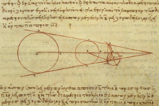
Among the first to find beauty as well as science in the universe were the Ancient Greeks, who began to deduce basic properties of the natural world and interpret the movements of the stars. Not only did they name most of the stars and record the groupings of stars into constellations that are still used today, they also created the basic words that astronomy uses, like galaxy-γαλαχτος (milky circle) ,

star – αστερι (star), astronomy- αστρονομος ( story of stars), among many others. Among their great scientists like Hypatia, Aristarchus, Ptolemy, Eratosthenes, and Democritus, were the discoverers of orbits, the knowledge the Earth was a sphere, the mapping of the stars, the recognition some stars (planets) were quite odd from the rest, and some texts that reference the possibility of a heliocentric solar system. But the Greeks also projected their myths and great stories onto the stars, highlighting the battles of Heracles, Orion, Perseus, Pegasus, the mythical beasts of old, like the Nemean Lion, Scylla, Cerberus, chimaera, bears, fish, dragons and Hydra, and tools that meant greatly to their civilization, like scales, triangles, and swords.

In another corner of the European continent, ancient Druid and pre-Germanic tribes, an ancient civilization created a grouping of immense stones that coincide with the movements of the sun, possibly used to tell the time of year as well as agricultural seasons.

This is Stonehenge, the English archaeological marvel that clearly demonstrates the culture’s analysis of the movement of the sun and clearly placing massive stones in a final place so they may serve as a tool to them and evidence of humanity’s fascination with that outside our atmosphere for generations to come.

Moving to another continent altogether, the Native Americans across North and South America interpreted celestial bodies in different ways and learned to analyze and interpret their movements to aid in measuring time, agriculture, and festivals of every kind. From Aztec sacrificial rites to Mayan Solar Calendars and Inca stones to highlight the different solstices throughout the year, these civilizations saw importance in the stars, interpreted them as messages from the gods, and preserved a deep understanding of the stars throughout their art and architecture.

As in the case of Teotihuacán, the ancient Mesoamerican city the Aztec found and renamed, giant buildings were made to align with the summer and winter solstices, these civilizations show an appreciation of the mathematics and order that govern much of celestial movement, as well as placing the stars in the highest regard possible.

North of the Aztecs, the Hopi Tribe of the Great Mesas of Southwestern North America also had a deep recognition of the stars in their art and culture.

This image illustrates Prophecy Rock, a record of the history and future of the Hopi people, identifying key points in their history, mainly the times of great change. This stone, illustrating the Sun and the stars, shows periods of human history, the foretelling of great calamities to the People, as well as the recounting of tragedies passed. Here the stars take on another meaning within the art and culture of a civilization, they are the foretellers of the future, images that identify the passage of time and the coming of change. This intuition is seen across many civilizations, who looked beyond the dirt and land they inhabit to see the immenseness that is found beyond a thin cap of gas, rather they entrusted their futures to that which always beyond their grasp.

Closer to the present, there are modern artists who also interpret the stars above. One of the clearest paintings of the starry night is, well, the Starry Night, by Vincent Van Gogh.

In the epitome of the Post-impressionist artistic movement, the stars above are focused on and detailed, the handiwork of God protecting the small town, the view of divine creation as the maximum exponent of art and beauty in the universe.

It is this same sky that inspired Van Gogh, Galileo, Copernicus, and so many other artists and scientists to pursue the nature of the stars, the twinkling points of beauty that entice us all to reach for them in an attempt to briefly glimpse them and understand them, including myself:

References:

http://www.davidreneke.com/aboriginal-astronomers/

https://camel76.wordpress.com/tag/constellations/

http://www.nationalgeographic.com/history/ancient/images/sw/stonehenge-from-above-692016-sw.jpg

http://www.proprofs.com/flashcards/cardshow.php?title=survey-art-history-art-263

http://science.nationalgeographic.com/science/archaeology/teotihuacan-/

http://www.twohawks.com/images/prophecyrock2.gif

http://uploads2.wikiart.org/images/vincent-van-gogh/the-starry-night-1889(1).jpg

A point of infinite space time curvature, or infinite density

We are bounded in a nutshell of Infinite space: Blog Post #8, Worksheet # 3.1, Problem #5: A point of infinite space time curvature, or infinite density.

5. \(M( < r)\) is related to the mass density \(\rho (r)\) by the integral: \[M( < r) = \int^r_0 4 \pi r^{2\prime} \rho (r^\prime) dr^\prime\] (Recall that the \( 4\pi r^\prime \) comes from the surface area of each spherical shell, and the \(dr^\prime\) is the thickness of each thin shell; talk to a TF if this is not clear.) The fundamental theorem of calculus then implies that \(4\pi r^2 \rho(r) = d M( < r) / dr\). For the case in question 4, what is \(\rho(r) \)? Is the density finite as \(r \to 0\) in the case of a flat rotation curve?

Using the several definitions offered for \(M( < r)\), we can begin to unravel the formula that would yield the relationship of stellar density in the galaxy to the total mass. Using the previous definition of \(M( < r)\), we have: \[ M( < r) = \frac{V_c^2 r}{G}.\] Yet we also have the equation for \( d M( < r) / dr\),

\[4\pi r^2 \rho(r) = d M( < r) / dr ,\] and if the derivative of the first equation was done, then these formulas could be equated. Thus, \[ dM( < r )/dr = \frac {d\frac{V_c^2 r}{G}} { dr} , \] \[ M( < r)^\prime = \frac{V_c^2}{G}, \] since the velocity of the galaxy is an established value as well as the gravitational constant, they are treated as constants when deriving and thus only since the velocity of the galaxy is an established value as well as the gravitational constant, they are treated as constants when deriving and thus only r is differentiated. The equations seen now equated through \( M( < r)^\prime \) would be:

\[4\pi r^2 \rho(r) = = \frac{V_c^2}{G}, \] which can be re written for \( \rho (r)\) : \[ \rho (r) =\frac { V_c^2} {4\pi r^2 G } ,\] which can now serve to inform us on the pattern of \( \rho (r)\) when \(r \to 0\). We can see that as r approaches 0, the value of the denominator becomes increasingly small, and thus the total value of the expression grows substantially, resulting in the conclusion that \( \rho (r)\) tends towards \(\infty\) as \(r \to 0\).

But it actually turns out to be flat…ish

We are bounded in a nutshell of Infinite space: Blog Post #7, Worksheet # 3.1, Problem #4: But it actually turns out to be flat…ish

4. We actually observe a flat rotation curve in our own Milky Way. (You will show this with a radio telescope in your second lab!) This means \(v(r)\) is nearly constant for a large range of distances.

(a) Lets call this constant rotational velocity \(V_c\) . If the mass distribution of the Milky Way is spherically symmetric, what must be the \(M( < r)\) as a function of \(r\) in this case, in terms of \(V_c\), \(r\), and \(G\) ?

(b) How does this compare with the picture of the galaxy you drew last week with most of the mass appearing to be in bulge?

(c) If the Milky Way rotation curve is observed to be flat \((V_c \approx 240 km/s ) \) out to 100 kpc, what is the total mass enclosed within 100 kpc? How does this compare with the mass in stars? Recall the total mass of stars in the Milky Way, a number you have been given in your first assignment and should commit to memory.

(a) Now that we redefined \(v(r)\) as \(V_c\), and \(M_{enc}\) will now be \(M( < r)\) , these new description will appear in the formulas used previously. Following this, we now start to understand the problem, we simply need to re-express the values set forth by the previous problem with new definitions and understand the interpretations. These equations now leave us with: \[V_c = \left(\frac{G M( < r)}{r}\right)^\frac{1}{2} ,\] \[\frac{V_c^2 r}{G} = M( < r)\] the form of the equation in its new iteration with the new definitions for the variables and outputs.

(b) However, as we start comparing the view of the Milky Way, as we saw in previous blog posts and readily available as part of your night sky if you have low light pollution and are in the southern hemisphere, and the mathematical models we have been using the last couple of problems, there seems to be a problem. We have been assuming the Milky Way can be considered a spherical galaxy when it clearly is not, rather it is a Spiral Barred galaxy that has become flat because of billions of years of rotations and conservation of angular momentum. This also conflicts with the fact we have been assuming symmetrical mass distribution when we are also aware of the fact of varying densities of the galaxies depending on the distance from the center.

(c) Now, taking into account the distance of 100 kpc where most of the mass of the galaxy is found, and the apparent speed of the curvature of the galaxy \((V_c \approx 240 km/s ) \), these values can simply be inserted into the equation to find the mass of the galaxy. First, a few constants: \[G_{(gravitational constant)}=6.674\times10^{-8}\frac{cm^3}{g s^2}\] \[2 \times 10^{23} \frac{g}{M_\odot }\] \[ 1 pc = 3.1 \times 10^{18} \frac{cm}{pc}. \]

Using these values, we may start to plug into the general equation, adding in some dimensional analysis conversion factors:

\[\frac{V_c^2 r}{G} = M( < r),\]

\[M ( < r)=\frac{(2.4 \times 10^2 \frac{km}{s} \cdot 10^5 \frac{cm}{km})^2 \cdot 10^2 kpc \cdot 3.1 \times 10^{18} \frac{cm}{pc} } {6.674\times10^{-8}\frac{cm^3}{g s^2}} , \]

\[M( < r)= 2.7 \times 10^{45} g , \]

\[M( < r)= \frac { 2.7 \times 10^{45} g } {2 \times 10^{23} \frac{g}{M_\odot} } , \]

\[M( < r)= 1.4 \times 10^{12} M_\odot .\]

Thus we have the calculation for the mass of the galaxy where its majority accumulates, however, it is a known quantity that the amount of stars in the galaxy equates to a mass of \( 10^{10} M_\odot \), so there is a difference of 2 orders of magnitude in this scale. Therefore, there is an enormous amount of matter in the galaxy that is not stars, it could be dust, planets, gases and many other forms of matter, but even high estimates of all the visible matter in the universe does not account for the total mass of the galaxy. Therefore, there is mass in the galaxy that, so far, cannot be observed, but its effects are evident and necessary to explain the speed the galaxy spins at the distances it does. This is dark matter, some unknown substance* in the universe that acts upon it without our being able to ascertain what it is, it could be dark, un-ignited stars, it could be huge amounts of rocks and dust that are in some way invisible, or it could be accumulations and existence of massive quantic particles that seemingly never interact with what we perceive as normal matter. And I thought we were just talking about flat galaxies instead of spherical ones, yet the spherical now starts to make sense when you think where all the extra matter might be.

The Milky Way is now a sphere (trust me)

We are bounded in a nutshell of Infinite space: Blog Post #6, Worksheet # 3.1, Problem #3: The Milky Way is now a sphere (wait for it)

3. Last time we approximated the shape of our Galaxy as a cylinder. This time it will be a sphere. If there are no other large-scale forces other than gravity (a good approximation in most galaxies), then an object’s orbit around the galactic center will be approximately circular.

(a) Show that Kepler’s 3^rd can be expressed in terms of the orbital frequency \(\Omega \equiv 2\pi / P \) (i.e. orbits/time) and the distance from the center \[r^3 \Omega^2 = GM_{tot} \]

(b) Now, assume that the Milky Way has a spherical mass distribution – this is a good approximation when talking about the total mass distribution. Using what you learned from Problem 2 (Gravitational Shell Theorem), rewrite the above for an object orbiting a radius r from the center of the galaxy.

(c) Next, let’s call the velocity of this object at a distance r away from the center, \(v(r)\). Use Kepler’s Third Law as expressed above to derive \(v(r)\) for a mass m if the central mass is concentrated in a single point at the center (with mass \(M_{enc}\), in terms of \(M_{enc}\), \(G\), and \(r\). This is known as the Keplerian rotation curve. As you saw earlier, it describes the motion of the planets in the solar system, since the Sun has nearly all of the mass.

(a) First off, let us establish what, exactly, is Kepler’s third law. As described by: \[P^2 = \frac{4 \pi^2 a^3}{ GM_{tot}} , \] the equivalency states how, depending on the semi major axis of the ellipse of the rotation of the celestial body (a) and the total mass of the object, the period of rotation changes. This same description of orbital period (P) can be expressed in terms of the orbital frequency, the amount of rotations in a given time. Using the equation \[\Omega \equiv 2\pi / P , \] for orbital frequency \(\Omega\), \(P\) can be solved for and thus get: \[ P \equiv 2\pi / \Omega , \] which can now be placed directly into Kepler’s Third Law Equation: \[(2\pi / \Omega)^2 = \frac{4 \pi^2 a^3}{ GM_{tot}} , \] and now solved for when the orbit approximates a circle and thus the semi major axis a is also the r of the circle,

\[\frac {4\pi^2}{\Omega^2} = \frac{4 \pi^2 r^3}{ GM_{tot}} , \]

\(4 \pi ^2\) is canceled on both sides and figures are cross multiplied,

\[ GM_{tot} = r^3 \Omega^2 , \]

Which is identical to the original equation the problem asked us to prove.

\[r^3 \Omega^2 = GM_{tot} \]

(b) What this problem refers to is the Shell Theorem, a description of astrophysical phenomenon, specifically gravity when great amounts of matter exist in an area, from a particular perspective. The shell theorem explains how, when an object is found in concentric circles (spheres in 3 dimensions) which all have matter, and thus gravity, then the particular object will feel only the gravity of the masses (shells) that are more inward than his present position. Thus the gravity of outside shells is negligible if existent, and all the gravitational force is felt towards the center of the gravitational shells.

If this idea is extrapolated for a spherical galaxy (as the problem describes), then the gravity any observer feels is only towards the center of the spherical galaxy, not towards that which is farther away from the center than the observer. This becomes an alteration for Kepler’s Third law equation we just saw, changing the \(M_{tot}\) to \(M_{tot} - M_{ext}\), and producing: \[r^3 \Omega^2 = G (M_{tot} - M_{ext}), \], and now describing \(M_{tot} - M_{ext}\) as the mass enclosed to the inner spherical shells \(M_{enc}\) we now have the equation: \[r^3 \Omega^2 = GM_{enc}, \] relating the Shell Theorem to the rotation of an object from the center of the galaxy.

(c) Now, to obtain \(v(r)\), the equation must be reworked with the knowledge of orbital velocities as well. Orbital velocity \(\omega\), which is the same as \(v(r)\), is defined by: \[\omega = \frac {2\pi}{P} r.\] In this iteration of the equation, the \(r\) is specifically separated to illustrate how the value of orbital frequency \(\Omega\) is clearly present in orbital velocity. The equation can now be re written as \[\omega = \Omega r,\] and can now be solved as \[\Omega = \frac{\omega}{ r}.\] Placed into the original Keplerian equation as:\[r^3 \Omega^2 = GM_{enc}, \] \[r^3 \left(\frac{\omega}{ r}\right)^2 = GM_{enc}, \] \[r \omega^2 = GM_{enc}, \] \[\omega^2 = \frac{GM_{enc}}{r}, \] \[ v(r) = \left(\frac{GM_{enc}}{r}\right)^\frac{1}{2} . \] This is the formula for predicting rotation curves and speeds of a galaxy.

Monday, September 14, 2015

Eye on the Supernova

We are bounded in a nutshell of Infinite space: Blog Post #5, Worksheet # 2.1, Problem #4: Eye on the Supernova

4. A supernova goes off and you can barely detect it with your eyes. Astronomers tell you that supernovae have a luminosity of \(10^{42} \frac{erg}{s}\) ; what is the distance of the supernova? Assume the supernova emits most of its energy at the peak of the eye’s sensitivity and that it explodes isotropically.

For this problem, it is especially important we start setting up some constants and numbers that might make little sense at first, but as the problem progresses, their use will become apparent. These values are: \[L_\star = 10^{42} \frac{erg}{s} , \] \[\lambda_{(Wavelength of Supernova Light)} = 500 nm = .5 \times 10^{-4} cm , \] by using the equation \(c= \lambda \nu \), the frequency of the light the supernova emits is: \[\nu = 5.96 \times 10^{14} s^{-1} , \] \[h_{(Plank’s Constant)} = 6.6 \times 10^{-27} erg \cdot s , \] \[Radius_{Pupil}= .433 cm\] \[Area_{eye} = \pi r_{eye}^2 = .589 cm^2 , \] \[n_{minimum photons the eye must receive}= 10 photons , \] and \[t_{eye exposure}= .1 s \] (the amount of time necessary for the eye identify a single image, so if more than 1 image is presented in a .1 s interval, the eye cannot recognize individual images, like in a movie).

With these values, we can begin to plug into values that will first lead to the amount of photons emitted by the supernova per second and later the actual distance of the observer from the supernova. The equation that describes the energy of 1 photon is: \[ E = h \nu , \] and this equation can be manipulated with \(E= \frac {L_\star}{n_{(Number of photons from Supernova)}}\) since \( \frac {L_\star}{n}\) is another way of describing the individual energy of a photon. Plugging in values:

\[\frac {L_\star}{n_{(Number of photons from Supernova)}} = h \nu ,\]

\[ n_{(Number of photons from Supernova)}= \frac {L_\star}{ h \nu} ,\]

\[ n_{(Number of photons from Supernova)}= \frac {10^{42} \frac{erg}{s}}{6.6 \times 10^{-27} (erg \cdot s) \cdot 5.96 \times 10^{14} s^{-1}} ,\]

\[ n _{(Number of photons from Supernova)} = 2.5422 \times 10^{53} \frac{photons}{s} . \]

With the number of photons emitted per second, this number can now be plugged into the photon flux equation: \[\frac{n}{4 \pi \delta^2} ,\] which, as you can see, describes the amount of photons emitted divided by the surface area the shell of continuous photons occupies at the distance \(\delta\) it has traveled.

This photon flux can also be calculated by understanding the amount of photons that are absorbed in the pupil in a given period, which is calculated with: \[\frac{n_ {minimum photons the eye must receive}}{A_{eye} t_{exposure}} .\]

And now these two equations are equalized since they are the same value: the photon flux, the photons in a specific area, \[\frac{n_{(Number of photons from Supernova)}}{4 \pi \delta^2} = \frac{n_ {minimum photons the eye must receive}}{A_{eye} t_{exposure}} ,\] and solve for the distance \(\delta\) from the observer to the supernova.

Now we solve for \(\delta\):

\[\frac{n_{(Number of photons from Supernova)} \cdot A_{eye} \cdot t_{exposure}}{4 \pi \cdot {n_{minimum photons the eye must receive}}} = \delta^2 , \]

\[\delta= \left( \frac{n_{(Number of photons from Supernova)} \cdot A_{eye} \cdot t_{exposure}}{4 \pi \cdot {n_{minimum photons the eye must receive}}}\right)^{\frac{1}{2}} , \]

to now start plugging in the values:

\[\delta= \left( \frac{2.5422 \times 10^{53} \frac{photons}{s} \cdot .589 cm^2 \cdot .1 s }{4 \pi \cdot {10 photons}}\right)^{\frac{1}{2}} , \]

\[\delta= 1.1 \times 10^{25} cm\] times the conversion factor of cm to pc

\[\delta= 1.1 \times 10^{25} cm \cdot \frac{1}{3.094 \times 10^18 \frac{cm}{pc}} , \] equals

\[\delta= 3.55 \times 10^6 pc .\] Which is how far away the Supernova is from your eye.

Means of Measuring Stars

We are bounded in a nutshell of Infinite space: Blog Post #4, Worksheet # 2.1, Problem #3: Measuring Stars

3. You observe a star you measure its flux to be \(F_\star\). If the luminosity of the star is \(L_\star\),

(a) Give an expression for how far away the star is.

(b) What is its parallax?

(c) If the peak wavelength of its emission is at \(\lambda_0\), what is the star’s temperature?

(d) What is the star’s radius, \(R_\star\)?

(a) As might be evident, this problem, in general, assumes you have completed a few previous exercises that explain in further detail the nature of these questions, so I will be recreating the necessary portions to fill in some of the data.

Now then, the apparent distance of a star that is being observed is directly tied to some of the most important astronomical measurement, Flux \(F_\star\) and Luminosity \(L_\star\), which in turn are directly correlated with one another. Furthermore, some more information on \(F_\star\) and \(L_\star\), is that, respectively, they have the units \(\frac{erg}{cm^2 \cdot s} \) and \( \frac{erg}{s} \) (in standard \(c \cdot g \cdot s\) notation). If you look closely at these units, you can see the only difference is that \(F_\star\) also contains a division by Area, the total area that the sphere of emitted photons have covered over a certain distance \(\delta\). \(L_\star\)’s units also indicate how it is simply energy over a set time, and if you remember physics class, that’s the same as Power, but only in luminous terms.

So if Flux is only Luminosity divided by an area, then the equation is truly that simple, producing: \[F_\star = \frac{L_\star}{4 \pi \delta^2},\] and in particular, \(4 \pi \delta^2\) representing the area of an expanding sphere with radius \(\delta\).

Next we take the equation we just had, \[F_\star = \frac{L_\star}{4 \pi \delta^2},\] and solve it for distance: \[4 \pi \delta^2= \frac{L_\star}{ F_\star },\] \[ \delta^2= \frac{L_\star}{ 4 \pi \cdot F_\star },\] \[\delta= \left(\frac{L_\star}{ 4 \pi \cdot F_\star}\right)^{\frac{1}{2}}.\]

And there you have an expression for the distance of the star from the observer, knowing the \(F_\star\) and \(L_\star\).

(b) A parallax is the difference in point of view of the observer which causes the background behind an object focused on to change. This slight change allows astronomers to measure distances of stars whose parallax is noticeable enough that a distance may be calculated from the triangle made by the Earth’s two points of view (vertexes) at two points in its orbit around the Sun, and the third vertex being the object observed. Parallaxes are measured in arc seconds, the unit below arc minutes and degrees, and when an observed object has a parallax of 1 arc second, the established distance is 1 parsec.

From this interpretation, a pattern starts to emerge, for every one arc second of parallax, there is one parsec of distance to the star, and for every 2 arc seconds of parallax (the change was much more noticeable), there is \(\frac{1}{2}\) parsecs. This indicates how parallax and distance are inversely related, described by: \[ p[''_{(arcsecond)}]=\frac{1}{\delta} [pc_{(parsec)}]\] which is analogous to the same formula in terms of radians and Astronomical Units (1AU = the distance from the Earth to the Sun): \[\theta [rad] = \frac{1}{\delta} AU\] where \(1 pc = 2 \times 10^5 AU\) since \(1 [radian] =2\times10^5 [''] \) .

(c) For this portion of the problem, the question refers to the derivative of the equation to calculate the radiation emitted from a blackbody, a classification for objects that are perfect emitter of thermal radiation. The original equation is:

\[F_{\lambda} (T)= \pi \frac{2 \left(\frac{c}{\lambda}\right)^2}{c^2} \frac{h \frac{c}{\lambda}}{e^{\frac{h\frac{c}{\lambda}}{kT}}} - 1 , \]

and after fully differentiating it, the equation becomes:

\[5 = {\frac{h c}{\lambda kT}} \cdot {\frac {e^\frac{h\frac{c}{\lambda}}{kT}}{\lambda e^{\frac{h\frac{c}{\lambda}}{kT}}-1}}\]

which reduces to \[5 = {\frac{h c}{\lambda kT}}\] since the rest of the equation becomes virtually 1 with almost any value plugged in.

Solving for \(\lambda\), and plugging in all the constants: \[c_{(Speed of Light)} = 2.98 \times 10^{10} \frac{cm}{s} , \] \[k_{(Boltzmann’s Constant)} = 1.4 \times 10^{-16} \frac{erg}{K} , \] and \[h_{(Plank’s Constant)} = 6.6 \times 10^{-27} erg \cdot s , \] we get: \[\lambda = \frac {0.2857 cm \cdot K}{T} \] where T is the temperature at the desired wavelength.

And if you were to look for the Maximum temperature that a blackbody would produce as according to the wavelength, then simply plug in the maximum wavelength into: \[T=\frac {0.2857 cm \cdot K}{\lambda_{Max}} .\]

(d) As to the star’s radius, \(R_\star\), there have been several equations and constants that can be combined by analysis of their units to give the desired length measurement. These values are:

\[L_\star = \frac{erg}{s} , \] \[\sigma_{( Stephen-Boltzmann Constant)} = \frac{erg}{ s cm^2 K^4} , \] \[T^4 = K^4 , \] (the multiplication of \(\sigma\) and \(T^4\) is the result of the integration of the equation to calculate the radiation emitted from a blackbody), and: \[4 \pi R_\star^2 = cm^2 , \] which describes the cross section of the star. So if all these numbers are put together and then solved for \(R_\star\), then we have:

\[L_\star = 4 \pi R_\star^2 \sigma T_\star^4 \]

\[R_\star = \left( \frac{ L_\star}{ 4 \pi \sigma T_\star^4} \right)^{\frac{1}{2}}.\]

Sunday, September 13, 2015

Just take a right at Messier 103

We are bounded in a nutshell of Infinite space: Blog Post #3, Worksheet # 1.2: Just take a right at Messier 103

Here we will be looking at views of the Milky Way Galaxy, the only home our home has ever known. First from the top and then from the side view. The Milky Way exhibits what astronomers refer to as a Spiral Galaxy, in part because its arms (marked on the top view map) exhibit a spiral shape that extends throughout the entire arm. This shape is actually very similar to the geometric figure called a Fibonacci Spiral, a figure whose sides are dictated by a sequence of numbers where the previous number is added to the present one to make the next term (but more on this in the links).

Top View of the Milky Way

Some of the key features of the Milky Way as seen from the top:

· Spiral arms: The Norma Arm, the Sagittarius Arm (whose Orion Spur is where our Solar System resides), the Perseus Arm, the Scutum-Centaurus Arm, and the Outer Arm.
The galaxy also has the Near 3kpc (kilo-parsec) Arm and the Far 3kpc Arm, which are the two arms very close to the inner bars (large groupings of stars) of the galaxy.
· Black Hole: Sgr A*, the center of our galaxy, a supermassive black hole
· Our Sun is located in the Orion Spur of the Sagittarius Arm, 8 kpc from the center of the galaxy
· Orion Nebula: This stellar beauty is an area of star formation where gases and basic atoms mix and bind to begin fusion and give birth to stars
· Hyades: The nearest open cluster of stars ( a group of close stars born from the same molecular cloud) to the Sun
· Messier 103: One of the farthest recorded open clusters (although many more are believed to exist) that sits on the Perseus Arm of the Milky Way
· The length (and approximately its width) of our galaxy is 30 kpc

Side View of the Milky Way