Translate

Monday, October 19, 2015

Pick your Galaxy

We are bounded in a nutshell of Infinite space: Blog Post #20, Hubble Galactic Tuning Fork: Pick your Galaxy

Ever since Edwin Hubble proved there were many galaxies instead of just one great one (see http://ay17-rcordova.blogspot.com/2015/10/the-great-debate-or-my-universe-is.html for the full story), observations of deep space have yielded more and more diversity in galaxies, none being exactly alike. But like good, inclined to organizing, humans we are, we developed a solid system of classification that fits for most of the galaxies astronomers observe regularly.

We've been discussing many different types of galaxies, such as elliptical and spiral galaxies, as is the case of Andromeda and the Milky Way, but these in turn can be subdivided even further. According to Hubble's observations, he created a system of galaxy classification that described elliptical, spiral, and irregular galaxies.

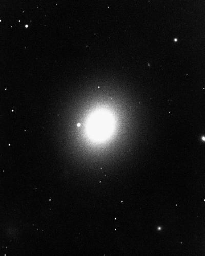
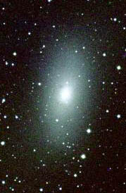
Starting with elliptical galaxies, which change from most "circular" to most elliptical, we have:

E0:

E1: 

E2:

E3:

E4:
E5:

E6:
E7:

And now we move on to Spiral Galaxies, starting with:

S0: 

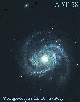
But here, the Spiral Galaxy classification splits off into barred and unbarred spirals. So unbarred Spirals look like: 

Sa:

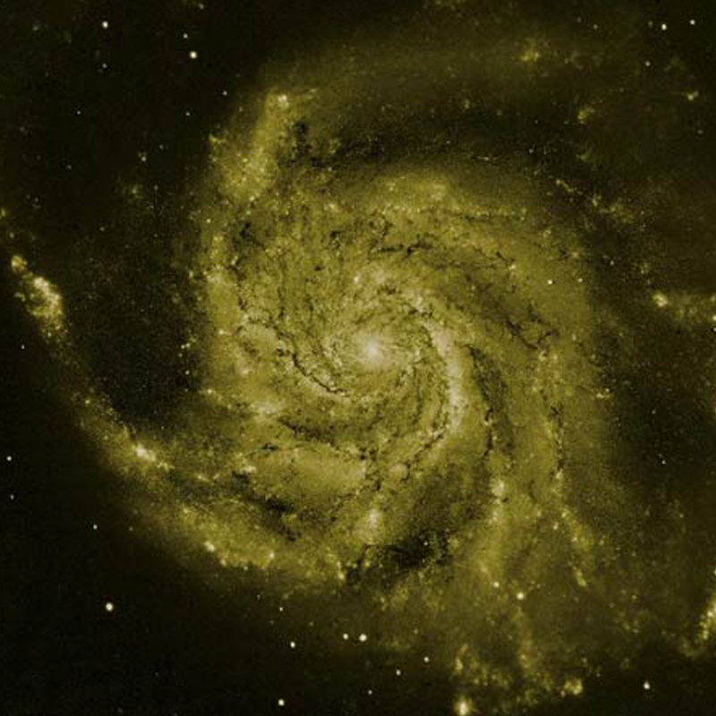
And they continue becoming more complex by adding to their amount of spirals and curvature,

Sb:

Sc:

And now for the barred Spiral Galaxies, which increase in complexity similar to the trend seen in unbarred spirals.

SBa: 

SBb: 

SBc: 

And finally there is a type of galaxy that fits into no classification: the irregular galaxies:

I: 

Although there are more galaxies that don't precisely fit into any of these classification, astronomers are starting to understand how galactic formation and evolution accounts for most of the shapes of these galaxies, including the irregular ones. Suffice to say, gas accumulates in a lot of ways, but when gas is the size of thousands of light-years, standard shapes start to emerge.

References:
http://www.newscientist.com/data/galleries/howdoesmygalaxygrow/m87cfht.jpg
http://www2.le.ac.uk/departments/physics/research/xroa/images/m87.gif/image_preview
http://www.astroimages.org/ccd/pics/m32-3.jpg
http://freestarcharts.com/images/Articles/Messier/M86_NASA_AURA_STScI.jpg
http://messier.seds.org/Pics/More/m49noao.jpg
https://www.le.ac.uk/ph/faulkes/web/images/m59.jpg
http://www.astronomynotes.com/galaxy/m110.jpg
http://bama.ua.edu/~rbuta/nearirs0/plate014c.jpg
http://www.mhhe.com/physsci/astronomy/fix/student/images/23f06.jpg
https://www.ualberta.ca/~pogosyan/teaching/ASTRO_122/lect23/ngc2997_aat.gif
http://www.astronomy.ohio-state.edu/~pogge/Ast162/Unit4/Galaxies/aat058.gif
https://upload.wikimedia.org/wikipedia/commons/thumb/c/c5/M101_hires_STScI-PRC2006-10a.jpg/1280px-M101_hires_STScI-PRC2006-10a.jpg
http://skyserver.sdss.org/dr1/en/astro/galaxies/images/n1300_SBb.gif
https://upload.wikimedia.org/wikipedia/commons/thumb/5/52/Hubble2005-01-barred-spiral-galaxy-NGC1300.jpg/350px-Hubble2005-01-barred-spiral-galaxy-NGC1300.jpg
http://www.stardoctor.org/M109-April2007-RubenKier-fullsize.jpg
http://www.robgendlerastropics.com/NGC4449-HST-GendlerS.jpg

Gas Makes a Trip Outside its Galaxy

We are bounded in a nutshell of Infinite space: Blog Post #19, Free Form #3: Gas Makes a Trip Outside its Galaxy

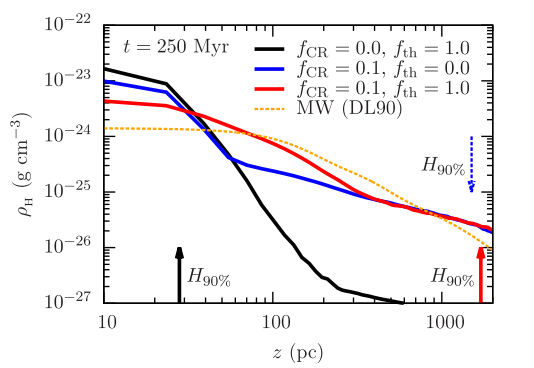
      In the paper “Launching Cosmic Ray-Driven Outflows from the Magnetized Interstellar Medium” by Philipp Girichidis et. al., they discuss more factors that drive galactic evolution and how these correct the present theoretical models to be more comparable to the observed data. In particular, the authors dealt with the formation of galaxies and the role galactic winds, cosmic rays, and thermal release shape the gas around and inside the galaxy. Defining some of the basic phenomenon we will see in this description, a main element of galactic formation is galactic wind, this immense force is present in galaxies from their formation and movement throughout the intergalactic medium, where gravity and more mass from accumulated gas cause these winds which give shape to the galaxy. 

These winds also make gas be ejected out of the galaxy, creating a gas halo around the galaxy. However, galactic winds are not powerful enough to account for all the gas that is seen outside the galaxies, rather another force was recognized to add a significant amount of force, the thermal missions from supernovae. As we know, supernovae are a type of star that grows to an incredible size and explode in the most amazing of ways, creating nebulae, incredible light emissions which outshine entire galaxies, and in some cases black holes.
Aside from the explosions themselves, these stars put out great energies in the form of thermal radiation, which also pushes the gas into a halo…but it still doesn’t fit the observed data. So, there must be another force that pushes the gas outside the center of the galaxy. This scientific group, located in part at the Max Planck Institute in Germany, found that cosmic rays, “high energy protons, electrons, and nuclei moving near the speed of light”, contribute significantly to the gas ejection. After these sources were all properly identified and their contribution to the gas movement weighed, the new theoretical projection matches up with the observed gas ejection.  
Black= Ejections from Thermal Energy;  Blue = Ejections from Cosmic Rays; Red= Combined Theo. Model; Yellow= Observed Data


All these measurements and continuations of experiments serve to illustrate how more and more experimental and theoretical scientists continue to work together within their fields to develop the best description and understanding of astronomical phenomenon. They find new and innovative ways to describe the way galaxies are shaped and the way they evolve, creating richer and more fundamental analyses of the process of interstellar formation. 

Reference:
http://astrobites.org/2015/10/01/cosmic-rays-make-for-windy-galaxies/

Sunday, October 18, 2015

Squiggle Math……………sure, why not

We are bounded in a nutshell of Infinite space: Blog Post #18, Worksheet # 6.1, Problem #4: Squiggle Math……………sure, why not
4. Over time, from measurements of the photometric and kinematic properties of normal galaxies, it became apparent that there exist correlations between the amount of motion of objects in the galaxy and the galaxy’s luminosity. In this problem, we’ll explore one of these relationships. Spiral galaxies obey the Tully-Fisher Relation: \[L \sim v_{max}^4\] , where L is total luminosity, and \(v_{max}\) is the maximum observed rotational velocity. This relation was initially discovered observationally, but it is not hard to derive in a crude way:
(a) Assume that \(v_{max} \sim \sigma\)(is this a good assumption?). Given what you know about the Virial Theorem, how should \(v_{max}\) relate to the mass and radius of the Galaxy?
(b) To proceed from here, you need some handy observational facts. First, all spiral galaxies have a similar disk surface brightnesses \((\langle I \rangle = L/R^2 )\) (Freeman’s Law). Second, they also have similar total mass-to-light ratio\(M/L\).
(c) Use some squiggle math (drop the constants and use \(\sim\) instead of =) to find the Tully-Fisher relationship.
(d) It turns out the Tully-Fisher Relation is so well-obeyed that it can be used as a standard candle, just like the Cepheids and Supernova Ia you saw in the last worksheet. In the B-band (\(\lambda_{cen} \sim 445 nm\) , blue light), this relation is approximately: \[M_B = -10 \log\left(\frac{v_{max}}{km/s}\right) +3 . \] Suppose you observe a spiral galaxy with apparent, extinction-corrected magnitude B = 13 mag. You perform longslit optical spectroscopy (ask a TF what that is), obtaining a maximum rotational velocity of 400 km/s for this galaxy. How distant do you infer this spiral galaxy to be?

(a) As established in the previous problem, “in observational astronomy, finding the velocity of any one, singular, small point, is both incredibly difficult, nigh impossible, as well as inefficient. It is much more useful to measure the combined velocity scatter of a system and use this value interchangeably in velocity equation to describe the total velocity of a large enough system.” And under this understanding, we can see why \(\sigma \) makes a good approximation for \(v_{max}\) for any large/diverse enough system. And now substituting \(v_{max}\) back into the final iteration of the virial theorem to find the relation of speed and mass , we get:   \[ v_{max}^2 \approx \frac{G (M) }{R} , \] taking away the constants, \[ v_{max}^2 \approx \frac{M}{R} , \] indicating a proportional relationship to M, and an inversely proportional relationship to R.

(b) This step merely establishes the proportions we will need in a bit. But taking the opportunity, we’ll explain the nature of squiggle math. This process bases itself not on actual numbers and cannot be used to find a definitive answer for any problem, rather it just states proportions and says one thing changes as the other changes, essentially. So if the problem describes how \[ \langle I \rangle = L/R^2 , \] so \[\frac{L}{R^2}\] and this is a proportion. In squiggle math, this would be represented by \[ L \sim R^2\] indicating the existence of this proportion. Another ratio given is (M/L), which means \(\frac{M}{L}\) which in squiggle math is \[M \sim L\]. These relationships are useful to understand the general physics of what is occurring in a problem, taking us to understand some key relationships in nature in very simple terms.

(c) Now, we can start using squiggle math to find the Tully-Fisher Relation, a simple representation of how two distinct physical properties of galaxies interact. Using what we have from part (a) and (b), we have: \[ v_{max}^2 \approx \frac{M}{R} , \] \[ L \sim R^2 , \] \[M \sim L ,\] and now these can be rearranged and combined. \[ v_{max}^2 \sim \frac{M}{R} , \] \[ v_{max}^2 R \sim M , \] \[ (M \sim v_{max}^2 R)^2 , \] \[ (M)^2 \sim v_{max}^4 R^2 , \]  which makes it easily changeable with a bit a squiggle math and the equations we had found just before, we have: \[ (L)^2 \sim v_{max}^4 L , \]  \[ L \sim v_{max}^4  , \]  which is exactly the Tully-Fisher Relation.

(d) For this problem, the Tully-Fisher Relation was already expanded on for us, and made into an equation that gives the absolute magnitude of a galaxy moving at a particular speed for a particular wavelength of light ( 445 nm in this case). This equation is: \[M_B = -10 \log\left(\frac{v_{max}}{km/s}\right) +3 , \] and using this with the distance modulus we used previously in Cepheid and Supernovae problems (http://ay17-rcordova.blogspot.com/2015/10/close-star-distant-star-near-starthat.html) \[M_{absolute} = M_{apparent} - 5 \times (\log_{10} (Distance )-1 ) ,\] we can find the distance of the galaxy once given the apparent magnitude, which is 13 in this problem.

Substituting the known value of 400 km/s rotational velocity, we have: \[M_B = -10 \log\left(\frac{400 km/s}{km/s}\right) +3 , \] \[M_B = -10 \log(400) +3 , \] \[M_B = - 23. \] Now that we have the Absolute and apparent magnitudes, we can solve for the distance to this galaxy. \[M_{absolute} = M_{apparent} - 5 \times (\log_{10} (D)-1 ) ,\] rearrange to solve for D, \[ 5 \log_{10} (D)- 5  = M_{apparent} - M_{absolute},\] \[  \log_{10} (D)  =\frac{ M_{apparent} - M_{absolute} + 5}{5},\] \[  D  =10^{\frac{ M_{apparent} - M_{absolute} + 5}{5}},\] and start plugging in: \[  D  =10^{\frac{ 13 - (-23) + 5}{5}},\]\[  D  =10^{8.2} ,\] \[  D  = 1.58 \times 10^8 pc ,\] \[  D  = 1.58 \times 10^5 kpc. \] The actual distance to the Spiral Galaxy. 

Energy in space is anything but one-dimensional

We are bounded in a nutshell of Infinite space: Blog Post #17, Worksheet # 6.1, Problem #3: Energy in space is anything but one-dimensional
3. One of the most useful equations in astronomy is an extremely simple relationship known as the Virial Theorem. It can be used to derive Kepler’s Third Law, measure the mass of a cluster of stars, or the temperature and brightness of a newly-formed planet. The Virial Theorem applies to a system of particles in equilibrium that are bound by a force that is defined by an inverse central-force law \(F \propto 1/r^{\alpha} \) It relates the kinetic (or thermal) energy of a system, K, to the potential energy, U, giving \[ K = - \frac{1}{2} U \]
(a) Consider a spherical distribution of N particles, each with a mass m. The distribution has total mass M and total radius R. Convince yourself that the total potential energy, U, is approximately \[ U \approx - \frac{GM^2 }{ R} \]  You can derive or look up the actual numerical constant out front. But in general in astronomy, you don’t need this prefactor, which is of order unity.
(b) Now let’s figure out what K is equal to. Consider a bound spherical distribution of N particles (perhaps stars in a globular cluster), each of mass m, and each moving with a velocity of \(v_i\) with respect to the center of mass. If these stars are far away in space, their individual velocity vectors are very difficult to measure directly. Generally, it is much easier to measure the scatter around the mean velocity if the system along our line of sight, the velocity scatter \(\sigma^2\) . Show that the kinetic energy of the system is: \[ K = N \frac{3}{2} m \sigma^2 \]  
(c) Use the Virial Theorem to show that the total mass of, say, a globular cluster of radius R and stellar velocity dispersion \(\sigma\) is (to some prefactor of order unity): \[M \approx \frac{\sigma^2 R}{G} . \]

(a) A simple relationship which continues to help coalesce information and difficult problems into understandable proportions, the Virial Theorem utilizes the correlation of potential and kinetic energies to describe the entirety of a large stellar system, such as that of a solar system or an entire galaxy. In this particular case, the Virial Theorem can be used to arrive at the velocity scatter of a galaxy as well as the relation this holds to mass.

First, we must find the relationship that gravitational potential energy has to the kinetic energy present in the system. Therefore, we begin with the basic Newtonian equation for the force of gravity from an object onto any other: \[ F_{Grav} = \frac{G (M_1 \cdot M_2)}{R^2} , \] (where G is the gravitational constant, the M’s are the objects’ masses, and R is the distance between them). This can be supplanted into the gravitational potential energy equation: \[U_{Grav} = - m\cdot g \cdot R ,  \]  \[U_{Grav} = - F_{Grav} \cdot R ,  \] \[U_{Grav} = - \frac{G (M_1 \cdot M_2) }{R^2} \cdot R ,  \] \[U_{Grav} \approx - \frac{G (M^2) }{R} , \] which is what the equation asks us to find and prove.

(b) In observational astronomy, finding the velocity of any one, singular, small point, is both incredibly difficult, nigh impossible, as well as inefficient. It is much more useful to measure the combined velocity scatter of a system and use this value interchangeably in velocity equation to describe the total velocity of a large enough system. Now then, the general equation for kinetic energy is: \[ K = \frac{1}{2} m_{Total} v^2 , \] and we know the total mass of a galaxy can be approximated with the amount of particles (objects) (N) times the median mass of each individual particle (m). Thus the equation becomes:  \[ K = \frac{1}{2} N m  v^2 , \] and now we introduce our definition of \(v\) in a large system: \[ K = \frac{1}{2} N m \sigma^2 , \] but this is still not the equation we are looking for. The coefficient of 3 is still missing, but what do we know exists in 3 dimensions (as far as we know): space! Not Space-Time, but rather just distance measurements, which corresponds to velocity vectors that exist in 3 directions/dimensions. Thus, the equation has to be added to the other two physical dimensions to make the entire energy equation: \[K_{Total} = K_x + K_y + K_z\] \[ K_{Total} = \frac{1}{2} N m \sigma^2  + \frac{1}{2} N m \sigma^2 + \frac{1}{2} N m \sigma^2 , \] \[ K_{Total} =\frac{3}{2} N m \sigma^2 .\]


(c) Therefore, taking both the equations we have just established (and in the case of K using it as only one dimensions since gravity is in one direction), we can now look for the relationship between speed and mass. Starting with \[ K = - \frac{1}{2} U , \] and substituting, \[ \frac{1}{2} N m \sigma^2 \approx - \frac{1}{2} \left(-\frac{G (M^2) }{R} \right) , \] and simplifying a bit, \[ M_{Total} \sigma^2 \approx \frac{G (M^2) }{R} , \] cancel out the M, \[ \sigma^2 \approx \frac{G (M) }{R} , \] and rearrange: \[ M_{Total} \approx \frac{ \sigma^2 R }{G} , \] the original equation we were looking for.  

Monday, October 5, 2015

The Great Debate (or, My universe is bigger than yours.)

We are bounded in a nutshell of Infinite space: Blog Post #16, History #1: The Great Debate (or, My universe is bigger than yours.)

In the early 20th century, astronomers Harlow Shapley and Heber D. Curtis began a discussion on the overall structure of the universe, essentially. Each posited different views on how the universe was constructed and the role of galaxies in it.


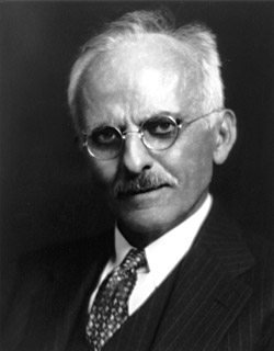
Harlow Shapley

Shapley postulated that the entire universe was the Milky Way Galaxy, one huge structure in the order of tens of thousands of light years across, and the farthest objects were globular clusters and the mysterious spiral nebulae. Shapley also believed our solar system is one that revolves around the galactic center, placing the Sun somewhere in the mid distance of the radius if our galaxy. He evidenced these claims with the measurements done with the Wilson telescope and how the data was analyzed and interpreted to mean how the light collected and the rate at which the image was processed evidenced a distance closer than what later experiments would prove. He also relied on the early understanding of Cepheid variables and misinterpreted their distance in finding out how far away the so called spiral nebulae were, although Cepheid data did lead him to make correct observations regarding the general order of the size of the galaxy.

Heber D. Curtis

On the other hand, Heber D. Curtis thought of a completely different system for the universe as a whole. He came to understand that the universe was made up of many galaxies, which could actually be the spiral nebulae that were routinely observed.  Using the data from telescopes around the world, Curtis saw that the spirals were definitely extra galactic objects, because of the fact of how small he believed the Milky Way to be and the observations of the spirals’ physical properties resembling many qualities already found in the Milky Way. He evidenced these claims by undermining the possibility that the spirals could be nebulae, citing many facts like spectrum analysis and luminosity distribution as reasons why there is no tenable way the spirals could maintain a shape and structure within a galaxy. He further postulates his “Island Universe Theory” where many spirals exist in the universe and we are one of many evidenced by how a galaxy like Andromeda would need to be extremely far away for it to be seen as it is, were it the size of our galaxy, and thus its speed at which it heads towards us makes more sense than if it were a “small” nebulae inside the galaxy. However, Curtis also posited that he also interpreted the data from the Cepheids that Shapley and other astronomers used, and found his to result in a smaller Milky Way Galaxy, and as such the solar system is closer to the enter, and quite near it according to his measurements.

Nevertheless, both of these men were right and wrong, about different aspects of their theories. In the mid 1920’s, Dr. Hubble searched for and found more conclusive evidence for the nature of the universe, employing measurements of Cepheid variables and other distance modulus to discover key attributes of the universe. He saw not only that the universe is actively expanding, but also how there were a seemingly infinite number of galaxies, as per Curtis’s theory, within our corner of the universe where the oldest light has gotten to us. Later on, experiments and observations of clusters and light absorption rates proved that the Milky Way is quite larger, in the same order of magnitude as Shapley’s hypothesis, and that we are inside one of the arms midway between the center and outer bounds of the galaxy. Essentially, they both won, they both contributed to the development of a general understanding of the composition of the universe (including hints of “invisible objects” that play into the mechanisms of the galaxy), and furthering the way astronomical would be interpreted for decades and now almost a century since their great debate.


Reference: http://apod.nasa.gov/diamond_jubilee/debate_1920.html

Supernovas be exploding

We are bounded in a nutshell of Infinite space: Blog Post #15, Worksheet # 5.1, Problem #4: Supernovas be exploding
4. Some stars explode as supernovae (SNe). In particular, Type Ia Supernovae come from exploding white dwarfs in binary systems. For now, it’s not important to know how this happens. It is, however, critical to learn the consequences of this mechanism, because they too are standard candles.
(a) As with the Cepheids, we can analyze the light curve of Type Ia SNe to standardize them. Below is a set of light curves. Examine them carefully, considering quantities like light curve shape, width/timescales, relative & absolute luminosity, &c. Find a rough relation obeyed by all the Supernovae Type Ia. Note: Although the supernova light curves have many features, try to relate just one of them to the peak magnitude. In other words, your relationship should have the form: \[M_{Max} = A* Feature + M_0 \] , where \(A\) and \(M_0\) are variables you should find.


(b) Describe how you would measure the distance to a Supernova Ia.
(c) Measure the distance to SN Cornell, whose light curve is shown below.

(a) Previously, we were looking at Cepheid variables, a type of star that allows astronomers to measure distances to other corners of the universe more easily than anything that could be done with a parallax measurement, but this is still not the farthest reaching measuring tool we have at our disposal. One of the farthest reaching tools in astronomy is the sight of type Ia supernovae. With these, exploding stars that outshine the entire galaxy when they occur, astronomers can measure the distances to incredibly deep space objects.

By analyzing the different characteristics of each light curve, there is a particular point that seems to repeat itself consistently: the period and Mean Absolute Magnitude of every star line up in the same place, the exact center of each plot, which means these could all be a set of data points for another type of graph that yields the relationship we could extrapolate to other Supernovae.
Checking every star and finding the exact mean magnitude by measuring the \(M_{Max} \) and \(M_{x_0 , y_0 } \) and getting their average \[\left(Half Max Magnitude = \frac {M_{Max} + M_{x_0 , y_0 }}{2}\right),\] and find the corresponding Period coordinate on these graphs, drawing lines on the graphs in the y value we just found and taking the corresponding Period value.
These values for the 4 Supernovae in the plots give us the following data:
SNe Name
Period
Max Absolute Magnitude
Harvard
44
-19.75
Princeton
42
-19.8
Yale
52
-19.25
Brown
48
-19.5

Which can now be used in the same analysis used previously when interpreting Cepheid variable data.
Creating a graph of the Supernovae values yields:
Which gives us an equation in the form of Ax + B that can be used for any number of situation to find the absolute magnitude of a star. Thus, the value of A is 0.057, while the value of \(M_0\) is -22.22, with a linear feature.

(b) Knowing a way to estimate the Max Absolute Magnitude by knowing the time when the Supernova will be at half its peak magnitude offers a very clear way for how its distance can be understood by simply knowing its light curve with apparent magnitude. By using the Magnitude-Distance equation used with the Cepheid problem, \[M_{absolute} = M_{apparent} – 5 \times (\log_{10} (Distance )-1 ) ,\] and solve for distance (in parsecs) when \[d = \left( 10^ {2 + 0.4 (M_{max apparent} - M_{max absolute})} \right)^(\frac{1}{2}\].

(c) Using the knowledge of an equation which yields the Max Absolute Magnitude of a Ia Supernova, we can apply the several equations to the light curve of the Cornell SNe. Measuring its apparent magnitude light curve it maxes out at 7.0, so the mid-max-magnitude here would be 8.5, as per our earlier equation. This magnitude then corresponds to a specific time, around 50 days, which can now be put into the equation. \[M_{Max} = A* Feature + M_0 ,\] \[M_{Max} = 0.057* t + -22.22, \] \[M_{Max} = 0.057* 50 + -22.22, \]
 \[M_{Max} = -19.37 .\]

With this number, we can plug it back into the distance formula: \[d = \left( 10^ {2 + 0.4 (M_{max apparent} - M_{max absolute})} \right)^(\frac{1}{2}, \]  \[d = \left( 10^ {2 + 0.4 (7 – (-19.37))} \right)^(\frac{1}{2} ,\] \[d = \left( 10^ {12.55} \right)^(\frac{1}{2} , \]\[d = 1879316.8 pc = 1.9 \times 10^3 kpc . \] The total distance to the Cornell Ia Supernova. 

Close star, Distant Star, Near Star….that just became a Far Star….

We are bounded in a nutshell of Infinite space: Blog Post #14, Worksheet # 5.2: Close star, Distant Star, Near Star….that just became a Far Star….
As we previously learned, Cepheid variables are a special class of stars that radially pulsate in a predictable way. In 1908, Henrietta Swan Leavitt discovered that there is a distinct relationship between a Cepheid’s luminosity and pulsation period by examining many stars in the Magellanic Clouds. Henrietta was a member of “Harvard’s computers,” a group of women hired by Edward Pickering to analyze stellar spectra and light curves. In this worksheet, we will use Henrietta’s original data set to find our own Period-Luminosity relation for Cepheid variables.
1. The data file, “Cepheid variables.csv,” contains data for 25 Cepheid variables located in the Small Magellanic Cloud (SMC). Each line contains a specific Cepheids: (1) ID number, (2) Maximum apparent magnitude, (3) Minimum apparent magnitude and (4) Period. Calculate the mean apparent magnitude for each Cepheid.
 2. The distance to the SMC is about 60 kpc, where kpc = 1000 pc. Convert your mean apparent magnitudes into mean absolute magnitudes. Plot the Cepheid mean absolute magnitudes as a function of period. This plot should look exponential.
3. It is often handy to plot exponential (or power-law) functions with one or more logarithmic axes, which “straightens out” the data. Magnitudes are already exponential, so we don’t need to adjust that axis. Plot the Cepheid mean absolute magnitudes as a function of \(\log_{10} Period\) . Verify that the plot now looks linear.
4. Now that the data look linear, we can estimate the parameters of a linear relation, \(M_V (P) = A\log_{10}(Period) +B\) . A and B are “free parameters” that allow the function to match the data.
5. BONUS: You can determine the precise values of A and B by minimizing the difference between the observed points and the model using the metric: where \[\chi^2 = \sum\limits_{i=1}^{25} (O_i – C_i )^2\] \(O_i\) is the observed value and \(C_i\) is the predicted (model) value.

We are now working with how astronomers measure extreme distances once tools like parallax become impossible to use. One way larger distances are measured is by finding clear examples of astronomical markers, objects in the sky whose characteristics are constant throughout the universe, whose traits can be analyzed and a correlation to distance and intrinsic properties can be found. Cepheid variables are a type of star that pulsate with light in a very predictable and measurable manner, and when many of these variables are compared and plotted, a distance formula emerges, as discovered by Henrietta Levitt.

In the case of this particular problem we have been presented with, we are going to go through the entire worksheet in one fail swoop, working it as individual components of a more complete system. Furthermore, some programming experience would definitely help with plotting and fitting the functions we will be seeing in this problem, but in any case we will be putting up all the code used, and brief explanations for what they do. So for this problem, we will be using some of the first data ever used to measure these Cepheid Variable Stars, which you can access through
and with it have data as prescribed by the instructions of the problem.

Using the magnitude-distance equation: \[M_{absolute} = M_{apparent} – 5 \times (\log_{10} (Distance )-1 ) ,\]  where the \(M_{apparent}\) is \[\frac{M_{max} + M_{min} }{2} , \] we can plot the values given in the file and see how these line up in a graph.

Up to know, we’ve had to use a lot of different measurements and formulas for calculating what leads to the solution to this problem, so let’s see the code that can help us find the answer: (%% indicates a comment, not part of the code)
import numpy as np
import math
import matplotlib
import matplotlib.pyplot as plt 
%%The basic Python introductions to the code, which allows for the use of mathematical and number systems, as well as a plotting element
c=np.loadtxt(fname='Cepheid_variables.csv', delimiter=',')
id, max, min, period = c.T
%%Presents the file (stored in the used computer) to the code and we give each column a name that will be used in later  equations.  
mean_apparent= (max+min)/2.0

mean_absolute = mean_apparent- 5.0*(math.log10(60000)-1)
%%The two equations we were seeing earlier, which establish the values used to plot the figure, with 60 times 1000 parsecs as the distance in the equation.
plt.figure(1)
%%This establishes that this is the first of other figures to be presented at the same time.
plt.plot(period, mean_absolute, "bo")
plt.xlabel('Period (Days)')
plt.ylabel('Mean Absolute Magnitude')
%%Now we use these commands to name the axes of our graph, give some color to definition to the set of points, and tell it to plot the exact values we have been finding with the previous commands, and finally plot it:


Next, we will begin analyzing the plot, and change it as necessary to find what we wish to extract form it. Basically, this means we have to adjust the period axis to it follows a logarithmic increase, and this convert what looks like an exponential or logarithmic function into a linear function. This is done in Python by writing:
plt.figure(2)

LogPeriod = np.log10(period) %% This changes the period into a logarithmic quantity
plt.plot(LogPeriod, mean_absolute, "bo")
plt.xlabel('Period (Days)')
plt.ylabel('Mean Absolute Magnitude')
%%And now we plot the figure again and get:

Now finally we can start interpreting the data by placing a linear fit to the data points and extracting the coefficients and constants A and B to find the complete description of Cepheid periods and magnitudes. We use the script:
A,B = np.polyfit(LogPeriod,mean_absolute,1) %%The linear fit of the equation defined…
plt.plot(LogPeriod, A*LogPeriod+B, "r")     %%...and placed

plt.show()       
%%The final command which plots all outlined figures and presents them as illustrations of the set of points

print(A,B)  
%%Tells the script to also print the values of A and B, the main question of the final problem. And with this, plots the final plot and values we have been looking for:
(A,B) = (-2.0331864794721257, -2.7275593585821594)


Altogether, the code looks like:
import numpy as np
import math
import matplotlib
import matplotlib.pyplot as plt
c=np.loadtxt(fname='Cepheid_variables.csv', delimiter=',')
id, max, min, period = c.T

mean_apparent= (max+min)/2.0

mean_absolute = mean_apparent- 5.0*(math.log10(60000)-1)

plt.figure(1)

plt.plot(period, mean_absolute, "bo")
plt.xlabel('Period (Days)')
plt.ylabel('Mean Absolute Magnitude')

plt.figure(2)

LogPeriod = np.log10(period)
plt.plot(LogPeriod, mean_absolute, "bo")
plt.xlabel('Period (Days)')
plt.ylabel('Mean Absolute Magnitude')

A,B = np.polyfit(LogPeriod,mean_absolute,1)
plt.plot(LogPeriod, A*LogPeriod+B, "r")

plt.show()


print(A,B)