Quick update, I went to JPL this Summer!!!!!!

I go to AAS!

The last few year have been a series of amazing experiences, and it has been incredible to spend this week presenting my research at the 231st Meeting of the American Astronomical Society! Check out the full text of the poster here!

This year

We are bounded in a nutshell of Infinite Space: Week 12: Free Form #17: This year

One more semester is about to end. I’ve been a year at Harvard, and it’s hard to believe 4 seasons have gone by. But this year has only gone by so quickly simply because of the sheer lack of pause. Every day, there are more than enough activities and events of every kind, be it presentations, classes, concerts, free food, or incredible opportunities. One such use of my time has been this class, Astronomy 16, an introduction to the physics of stars, planets, and the formation of the individual objects we study. After taking astronomy 17 last semester, I guess I had a bit of an insight going into the class, being less daunted by most of the material, and comfortable with the style of the class.

This being said, the difficulty between the courses was hardly noticeable, both requiring different approaches to learning and facing different kinds of problems astronomy is constantly berated with. From finding ways to cope with a huge source of light blocking our view for most of the day (Thank you, Sun, we love you (and need you to survive)), to coming to terms with only seeing the past as we look at the stars, Astronomy certainly has its unconventional problems. Furthermore, the portions of astronomical thought which deal with these realities (so pretty much all of it), are my favorite parts of the discipline. Throughout the semester, we consistently dealt with the origin of the light we see, stars and other objects which tell us how “life” (?) is in other sectors of the cosmos, and understanding the radiative processes have been my favorite components of the semester. However, I need to give a shout out to binary and locked systems, because actually observing one during a lab project and the exoplanet challenge was amazing!

Hello Mr Planet!

The most difficult parts of the semester would probably be the portions of the class when quantum mechanics, astrochemistry, and similar topics which became very abstract. Notwithstanding, I enjoyed these portions as much as the rest of the class, understanding these components to be integral in comprehending the way all the processes of astronomy work and the way we are currently able to observe anything at all. Without a doubt, this semester became easier than the last one had been, in part I am sure because of just being here longer and knowing what pace needed to be kept, but also because I’ve started to feel more comfortable, more at home in this occasional frozen-over hell, but truly hopeful of the next stages of college life, and learning more and more about this strange and beautiful universe we inhabit.  

I'll let the pictures do the talking

We are bounded in a nutshell of Infinite Space: Week 11: Free Form #16: I'll let the pictures do the talking 

 Stephen Hawing came to Harvard. Possibly one of the most influential physicists, cosmologists, science promoters, writers, of the last century, Dr. Hawking is a true stalwart. Not only because of his disability and the drive it takes to continue living and working to change the world, he is an unadulterated view of someone who has fought every step of the way to finally be the top in their field. Now, he came to Harvard as part of the opening of the Black Hole Initiative (hopefully I get a chance to work there for a while), where mathematicians, physicists, philosophers, and astrophysicists will work on better understanding the nature of black holes and the important role they play for the universe. Professor Hawking, on his part, went on to give a full lecture on quantum black holes. He started out with the basic premises, the nature of general relativity and space time, to later move on to the more interesting portions. The talk shifted to Schwarzschild, the dawn of the theory of black holes, and then to Richard Feynman and Arthur Penrose, people who further developed the theory and saw the consequences of black holes on structure formation. 

He then spoke of the components of black hole theory he had established in the past, especially the understanding of how black holes begin to fade due to radiation emission, called Hawking Radiation. This allows for a black hole to disappear after a great deal of time, but in this come the theoretical and frontiers of new black hole science: information theory. This aspect of black holes, thought up by Hawking, Strominger, and Perry, attempts to explain how black holes are a way that, originally, information could be completely vanished from the universe. Imagine you were to place an encyclopedia into a black hole, all the pages with all their facts would fall towards the singularity, ripped apart by tidal forces and spaghettified (for not humongous black holes), never to be seen again in our universe (yes, he got into the idea that black holes could very well be a gateway to another dimension). However, this is where the idea becomes very interesting, for black holes grow larger and their radius expands as they become more massive, as more things are thrown into it, and as the black hole eventually radiates out its existence, in theory the information first lost beyond the event horizon could come back in the form of thermal energy, technically not impossible to be turned into physical matter with all the pages on the Rhine, rhinitis, and rhinoceroses. If you want to learn more on how these black holes become the unification of quantum mechanics and general relativity, one of the main pursuits of modern physics. 

A Night at the Observatory

We are bounded in a nutshell of Infinite Space: Week 11: Free Form #15: A Night at the Observatory

Oh to be doing the Exoplanet Challenge. Here I am, awake during the daytime after being conscious throughout the night, and the weight on my eyelids is as strong as its ever going to be, and the fact I tried reading Plato this morning for my Ancient Greek class didn’t help at all. These are the thoughts that echo after spending last night (this morning) looking at HAT P 37b, a transiting exoplanet crossing in front of a star found in the Draco Constellation. As part of the Astronomy 16 course, we have the option of taking on the Exoplanet Challenge, a chance to use some of the more advanced tools available to undergraduates to try and find evidence of a planet crossing in front of a star we are observing. The challenge gives the unique opportunity of having to go up to the 8th floor of the Harvard Science Center, open the Astronomy Lab, and start prepping for the use of the Clay Telescope, all on our own (in groups of 2 or 3). As such, my partner and I went up to the telescope at midnight, set up all the systems, and waited until we had the data to be analyzed to find evidence of the transit and understand what it means. However, around 4:30 am, as we made the second batch of warm water for tea and coffee, we started comparing the photometry (brightness signatures) from the stars, waning to be sure we had indeed looked at the right object. As we plotted the graph, we could hardly make sense of the data, it shifting several times and having strange reference stars of which the main object’s signature was calculated by the software. We were lost for a bit. Soon after, around 5:30 am, the Sun started coming up on the horizon, and as such we started closing up shop and preparing to leave to a proximate future of a couch somewhere near. Leaving, we weren’t sure we had done it correctly, even though there was no step we could have missed, and we worried over having to go through this ordeal again.  

All this being said, we definitely lucked out with weather. And as we spoke coming out of the building, we knew there were slight places to grow and be more precise. We also understood that there was a definite value to being in the observatory all night, seeing how the sky moved throughout the night, and having the lab became not only be workspace, but starting to see it and the telescope as an extension of our senses. We grew to appreciate the instrument, and be fond of it the way one is of ones hands and eyes, but now having a dear appreciation of how they allow us to peer into the unknown. Ultimately, we were able to fix the data analysis, seeing as how we were using bad stars as references, and with the correction we could now clearly make out the light curve of the planet transit, the white whale we had been hunting throughout the night, with a better understanding of how difficult the job of the hunting sea captain, the searching astronomer, is, and what he can become.

Squiggle Math III, The Time Conundrum

We are bounded in a nutshell of Infinite Space: Week 11: Worksheet #20: Problem #2: Squiggle Math III, The Time Conundrum

2.

a. Time for some more squiggle math!! So from the previous problem on this worksheet relating temperature, luminosity, and the distance between the star and the object, we can rewrite it in terms of its variables as: \[ T \sim L_\star^{1/4} a^{-1/2},\] but since the temperature we can consider it to be constant for the purposes of this problem, we find that:  \[ a^{1/2} \sim L_\star^{1/4}\]

b. We can take the previous result relating the temperature to the distance, and find the relationship is also: \[ a^2 \sim L .\] Also, we know from a previous worksheet we did a couple of months ago that luminosity and mass are inherently linked in a star, which can be described with its proportion as:  \[ L \sim\ M^4,\] and by plugging these in, we find that:  \[ a^2 \sim M^4\] \[ a \sim M^2,\] which means \[ a_{HZ} \sim M_\star^2 ,\] where the looked for variable becomes: \[ \alpha = 2\]

c.  Furthermore, we can use these proportions to establish how Kepler’s third law works according to squiggle math: \[ P^2 = \frac{4\pi^2 a^3}{G M_\star}, \] becomes \[ P^2 \sim \frac{a^3}{M_\star} ,\] and according to our previous part, we can substitute in and find that: \[ P^2 \sim \frac{M_\star^{2^{3}} }{M_\star},\] which means \[ P^2 \sim M_\star^5\] \[ P \sim M^{5/2}.\]

Now, we want ot find the period of the Earth if the Sun were half its current mass, such that: \[ P \sim \left(\frac{1}{2} M_\star \right)^{5/2} ,\] turns into  \[ P \sim {\frac{1}{2}}^\frac{5}{2} M_\star^{5/2}\] \[ \sqrt{32} P \sim M_\star^{5/2},\] which means the new Earth period is related to the original period by:  \[ \frac{1}{\sqrt{32}} P_\oplus = P_{\frac{1}{2} M_\star },\] and thus, the Period of rotation becomes \[  P_{\frac{1}{2} M_\star} = \frac{365}{\sqrt{32} } = 64 ~days,\] our new definition of a year.

This is where you live

We are bounded in a nutshell of Infinite Space: Week 11: Worksheet #20: Problem #1: This is where you live 

1.

a.

b. For this problem, we are attempting to find the range of the distance around a star in which a planet may have liquid water, what we know as the habitable zone. In order to understand this, we must find the correlation of temperature and the brightness of stellar objects. For a planet, we know the Flux it receives from the star it orbits is: \[ \frac{L_\star}{4\pi a^2}  = F_P ,\] which can be re written to better represent all the energy impacting the planet in a specified time: \[ F = \frac{Energy}{time \cdot area}\] \[   \frac{L_\star}{4\pi a^2} \cdot \pi R_P^2 = \frac{Energy}{time}~received~by~planet\]

Furthermore, we should understand the energy the planet then radiates back into space, which can be described with the equation for bolometric flux: \[F = \sigma T_P^4,\] and from previous worksheets we know that the flux can be turned into luminosity by just multiplying by the surface area \[ L_P = \sigma T_P^4 \cdot 4\pi R_P^2\]  

c. Next we set these equations equal to each other and find the expression for the temperature of the planet: \[   \frac{L_\star}{4\pi a^2} \cdot \pi R_P^2 = \frac{Energy}{time}~received~by~planet = L_P = \sigma T_P^4 \cdot 4\pi R_P^2\]  \[   \frac{L_\star}{4\pi a^2} \cdot \pi R_P^2 = \sigma T_P^4 \cdot 4\pi R_P^2,\] we start simplifying the equation and find that \[ \frac{L_\star}{4a^2} = \sigma T_P^4 \cdot 4\pi ,\] which finally turns into: \[ T_P = \left(\frac{L_\star}{16 a^2 \pi \sigma}\right)^{1/4}\]

Also, we can keep on simplifying the expression were we to consider the definition of the star’s luminosity: \[L_\star = 4\pi R_\star^2 \cdot \sigma T_{eff}^4,\] which can be placed into the equation we just derived to further understand the factors involved: \[ T_P = \left(\frac{4\pi R_\star^2 \cdot \sigma T_{eff}^4}{16 a^2 \pi \sigma}\right)^{1/4},\] \[ T_P = \left(\frac{ R_\star^2 T_{eff}^4}{4 a^2 }\right)^{1/4},\] This results in the simplified version of the equation which expresses the relationship between the planet’s temperature, and the radius and temperature of the star: \[ T_P = T_{eff} \sqrt{\frac{R_\star}{2a}}\]

d. As we can see from the equations, the radius of the planet becomes insignificant, it not being a factor in establishing the temperature of the planet, rather the radius of the star comes into play.  

e. Now, we can assume some energy gets reflected from the surface, yielding an equation similar to: \[ T_P = \left(\frac{L_\star}{16 a^2 \pi \sigma}\right)^{1/4},\] but where A is the energy per time reflected: \[ T_P = \left(\frac{L_\star - A}{16 a^2 \pi \sigma}\right)^{1/4},\] which simplifies to: \[ T_P = T_{eff} \sqrt{\frac{R_\star}{2a}} - \left(\frac{A}{16 a^2 \pi \sigma}\right)^{1/4}.\] Therefore, the temperature most definitely goes down as the reflectivity increases.  

Molecular Clouds

We are bounded in a nutshell of Infinite Space: Week 10: Reading #8: Molecular Clouds

One of the most vital systems which led to our development as a solar system and eventually as a planet is the molecular cloud. These giant consolidations of gas condense and compact all kinds of elements left over from previous stellar formations and explosions, along with the interstellar medium, to have enough mass to eventually collapse into denser systems. These molecular clouds are the basis of the formation of all the structures we have been seeing in the past couple of weeks, planets, stars, moons, asteroids, and all the different structures of solar systems, all come from these incredible structures with the potential of creating all the diversity we have begun to see in looking at distant planets and other star systems. 

Furthermore, these molecular clouds collapse by a process of gravity overpowering the force of Pressure in the system, allowing for a runaway collapse into the more concentrated system. This process could yield several star systems close to one another, as well as other, more complicated structures such as two sets of binary stars orbiting one another. From the runaway collapse (better explained in http://ay16-rodrigocordova.blogspot.com/2016/04/stars-from-molecular-clouds.html ) we have denser groups of material which produce enough pressure and gravity to begin nuclear fusion at the core of the proto-star, to begin gaining material and influence the creation of the eventual protoplanetary disk.

Reference:

Chapters 5.1 and 5.3 of

Maoz, D. (2007). Astrophysics in a Nutshell. Princeton: Princeton University Press.

https://www.youtube.com/watch?v=YbdwTwB8jtc

The Best of all Newcomers

We are bounded in a nutshell of Infinite Space: Week 10: Free Form #14: The Best of all Newcomers  

Within the bounds of space news, you can’t get much more interesting than advances in rocket technologies and new and exciting ways of how we will continue getting to space. One huge advancement in the past months and years has been the development of private space companies, dedicated exclusively to the research and development of finding more affordable ways of getting to space and using existing and future technology to arrive at the goals of our exploration. One such company is SpaceX, founded by Elon Musk in 2002. A newcomer in the realm of aerospace corporations inhabited by titans like Lockheed Martin and Boeing, SpaceX boasts some of the most impressive technological improvements on space flight seen since the great pushes of innovation in the early days of the space race. In fact, just last weekend the pioneers successfully landed a spent solid rocket booster, after it was jettisoned by the payload arriving to the International Space Station, onto a barge-drone which successfully positioned to receive the incoming rocket, from SPACE. 

These are the frontiers of science fictions which are pushed today, the incredible feats which will push humanity towards new eras of exploration and discovery. Furthermore, SpaceX is developing several rockets to establish the future of space-travel, specifically the Heavy Falcon Tri-Booster Rocket system which will launch the missions SpaceX expects to send in the future. 

However, for all incredible feats SpaceX has accomplished, it still maintains a critical problem when considering how they expect to mount an expedition to Mars. Fundamentally, they are a company, and no matter the advances and loose capital, there is not free reign on the part of true visionaries for the future, as I believe Elon Musk to be, to simply go in pursuit of scientific discovery, for there is no revenue in sending people to Mars. However, SpaceX is developing the technologies which rival if not beat the established companies’ technologies, and as such could become the primary aerospace company for space agencies in the near future, as it has become for NASA in sending payloads to the ISS. Regardless of the scientific prospects of SpaceX, the fact remains they are pushing the boundaries of science and engineering, and as such will be crucial in the dawn of interplanetary travel, but until groups as “free” as NASA to explore scientific questions, with less accountability to stockholders and boards, are able to prepare, train, and develop the missions which take us to Mars, I doubt private sectors would be able to do anything similar. For it was not the Medici Bank which sent Columbus to America, but rather the Kings of Spain, people with enough free capital to see the value of exploration, beyond the scope of returns.

References: 

https://www.youtube.com/watch?v=4Ca6x4QbpoM

https://www.youtube.com/watch?v=sYmQQn_ZSys&ebc=ANyPxKpmf6gjojs_KZuAqsNVI4cFh3G29cFQE7wQ72Dg205rJS2P254XVMhGUQnJHqBjpBq8NHNojel9zEE7ZrQ7OC4R4_HZUw&nohtml5=False

http://www.latimes.com/business/la-fi-spacex-rocket-20160411-story.html

The Future of Space Travel

We are bounded in a nutshell of Infinite Space: Week 10: Free Form #13: The Future of Space Travel

The next stages of space travel is one we all share, something which is entrusted to our generation, our birthright, and our future. But, we will only get to the future by standing on the shoulders of giants, to quote Stephen Hawking. As such there is already a great deal of work being done to prepare humanity for our future among the stars, much of which is owed to the National Aeronautics and Space Administration. Nowadays, NASA is preparing for the next great step for mankind, the arrival of humans to a completely different planet, Mars. But this is hardly accomplished in a single day, rather years have gone into the making of the technologies which will propel us (literally) to the red planet. One such innovation which is currently being tested and prepped for its missions to deep space is the Orion Spacecraft and the Space Launch System (SLS). These products of ingenuity are the basis for our future among the stars, Spacecraft able to support humans on the longest voyages since the era of exploration some centuries ago. Orion will be the actual module astronauts will travel in to arrive on Mars, having facilities for life support as well as modules for propulsion and a Launch Abort System which would mitigate the dangers of the most perilous part of spaceflight, getting off the ground. 

Additionally, the SLS is an impressive cohesion of several solid rocket boosters and fuel tanks which make it the most powerful rocket in history. The SLS will be the rocket which launches Orion on its missions to our neighboring planets, giving it enough power to Orion to slingshot around the Moon, and ride along till arriving at Mars. Furthermore, there are other technologies just beyond the horizon which will change our views of space travel forever. Just think of ion propulsion, orders of magnitude more efficient than the traditional chemical propulsion, using ionized electrons from Xenon and other elements to produce the thrust which will propel future missions. Not only this, new technologies like Solar Sails and other fuels and propellants are the future of our exploration and further understanding of our stellar backyard. After all, if we don’t find ways to continue moving, eventually we won’t have a planet to call home simply because the Sun will explode in a fair amount of time, but staying on Earth is not the ultimate future for humanity, of that I am sure.

References:

http://spaceflight101.com/spacecraft/orion/

http://www.nasa.gov/centers/glenn/about/fs21grc.html

http://www.nasa.gov/multimedia/imagegallery/image_feature_2416.html

 http://www.nasa.gov/sites/default/files/atoms/files/sls_october_2015_fact_sheet.pdf

http://www.nasa.gov/sites/default/files/617409main_orion_overview_fs_33012.pdf

Where's that moon?

We are bounded in a nutshell of Infinite Space: Week 10: Worksheet #18: Problem #1: Where's that moon?  

1. Hill spheres. One outcome of planet formation is systems of satellites around planets. Now you may ask yourself, why do some planets have moons 10s of millions of kilometers away, while the Earth’s moon is only 400,000 km away. To answer this question we need to think about how big of a region around a planet is dominated by the gravity of a planet, i.e. the region where the gravitational pull of the planet is more important than the gravitational pull of the central star (or another planet).

a) Gravitational forces. Put a test mass somewhere between a star of mass \(M_S\) and a planet of mass \(m_P\) at a distance \(r_P\) from the star. Make a drawing marking clearly these characteristics as well as the distance r between the test particle and the planet. Write separate expressions for the gravitational force on the particle from the star and on the particle from the planet. At what distance r from the planet are the two forces balanced? This distance approximates the radius of the Hill sphere, which in the case of planet formation is the sphere of disk material which a planet can accrete from.

(b) Planetary Hill radii. Calculate the Hill radii for Earth, Jupiter, and Neptune. How do they compare with the separation between the planets and their most distant moons? 

a. With these hill spheres, the defining characteristic is the point of equilibrium at which the point mass would be find between the two masses. This is expressed with the law of universal gravitation: \[ F_{G_{r_P}} = F_{G_{r_P - r}} ,\] and reconfiguring these equations, we find how: \[ \frac{G M_S m_{part} }{(r_P - r)^2} = \frac{G m_P m_{part}}{r^2}\] \[\frac{M_S}{(r_P - r)^2} = \frac{m_P}{r^2} \] \[\frac{r^2}{(r_P - r) ^2} = \frac{m_P}{M_S},\]  which can be further simplified till finding: \[ \frac{r}{r_P - r} = \sqrt{\frac{m_P}{M_S}}\] \[ r = \sqrt{\frac{m_P}{M_S}} (r_P - r)\] \[ r(1+ \sqrt{\frac{m_P}{M_S}}) = \sqrt{\frac{m_P}{M_S}} r_P ,\] and thus we have \[ r = \frac{\sqrt{\frac{m_P}{M_S}} r_P}{ 1+ \sqrt{\frac{m_P}{M_S}}},\] which can be given a final derivation till a fairly simple relationship emerges: \[ r = \frac{\sqrt{m_P} r_P }{ \sqrt{M_S} + \sqrt{m_P}}\]

b. Now, we can take the equation we have found and find the hill radii for several planets in our solar system. But first, let us define a couple of values, such as the mass of the Earth: \[M _\oplus = 5.9 \times 10^{24} kg \] \[ M_\odot = 2 \times 10^{30} kg,\] and therefore: \[ 1 ~M_\odot = 3.3 \times 1- ^5 M_\oplus ,\] similarly: \[ 1 ~AU = 1.5 \times 10^8 km\]

First, for the Earth itself, we can find its hill radius: \[ r_\oplus = \frac{\sqrt{M_\oplus} r_P }{ \sqrt{M_S} + \sqrt{M_\oplus}},\] plugging in values, we find that: \[ r_\oplus = \frac{\sqrt{1 M_\oplus} (1 ~ AU) }{ \sqrt{3.3 \times 10 ^5 M_\oplus } + \sqrt{ 1 M_\oplus}} ,\] \[ r_\oplus = \frac{1}{5.7 \times 10^{2}}\] \[ r_\oplus \approx 2 \times 10^{-3} AU \approx  3 \times 10^5 km, \] and comparing it to the radius at which the Moon is found, we see that the hill radius we have calculated is similar to the actual distance to the Moon to a factor less than 2.

Now for Jupiter. Following the same process, we find that: \[ r_{Jup} = \frac{\sqrt{M_{Jup}} r_P }{ \sqrt{M_S} + \sqrt{M_{Jup}}},\]  \[ r_{Jup} = \frac{\sqrt{320 M_\oplus} \cdot 5.2 ~AU} { \sqrt{3.3 \times 10^5 M_\oplus } + \sqrt{ 320 M_\oplus } },\] which means the hill radius is \[ r_{Jup} \approx 0.15 AU \approx 2.2 \times 10^7 km ,\] which which is practically the same as the actual distance to (one of) the moons of Jupiter, \(2.4 \times 10^7 km\).   

And finally Neptune, the hill radius is: \[ r_{Nep} = \frac{\sqrt{M_{Nep}} r_{Nep} }{ \sqrt{M_S} + \sqrt{M_{Nep} } }\] \[ r_{Nep} = \frac{\sqrt{17 M_\oplus} \cdot 30~ AU}{ \sqrt{3.3 \times 10^5 M_\oplus } + \sqrt{17 M_\oplus}  },\]  and therefore it results in:\[ r_{Nep} \approx 0.2 ~AU \approx 3 \times 10^7 km,\] which is but a factor less than two away from the precise measurement of Neptune’s moon’s distance.   

Where does all the momentum of the spinning protoplanetary disk go?

We are bounded in a nutshell of Infinite Space: Week 10: Worksheet #17: Problem #1: Where does all the momentum of the spinning protoplanetary disk go? 

1. Angular momentum. In this problem we will obtain some intuition on why a disk must form during star formation if angular momentum is to be preserved.

(a) Cloud angular momentum. Consider a typical interstellar cloud core that forms a single star. You can assume it has a mass of \(1 \M_\odot\) and a diameter of 0.1 pc. A typical cloud rotational velocity is 1 m/s at the cloud edge. Calculate the angular momentum of the cloud assuming constant density. If the core collapses to form a Sun-like star, what would the velocity at the surface of the star be if angular momentum is conserved? How does this compare with the break-up velocity of the Sun which is \(\sim\) 300 km/s?

(b) Disk angular momentum. Assume that all the angular momentum is instead transferred to a disk of size 10 AU and negligible height. How massive must the disk be? You can assume constant density. (Hint: You can assume that the disk rotates with a Keplerian velocity given by \(v = \sqrt{GM/r}\) where M is the mass and r is the radius.)

c) Solar System. The Sun has a surface rotational velocity of \(\sim\) 2 km/s at the equator. How do the angular momenta of the Sun and Jupiter compare?

a. First off, let us lay out all the base data and equations we’ll need: \[v = 1 m/s \] \[ \omega = \frac{v}{R}\] \[R = 0.05 pc = 1.5 \times 10^{15} m\] \[ R_\odot = 7 \times 10^8 m\] \[M_\odot = 2 \times 10^{30} kg ,\] and the equation for angular momentum:  \[ L = I \omega .\]

Now we expand this for a sphere, and set the angular momentums equal to one another in order to find the rotational velocity: \[L = \frac{2}{5} M R^2 \omega,\] \[ L_{cloud}= L_\star,\] \[\frac{2}{5} M_\odot (0.05 pc)^2 \frac{1 \frac{m}{s}}{1.5 \times 10^{15} m } = \frac{2}{5} M_\odot (R_\odot)^2 \omega_\star.\] Now it’s just a matter of plugging in the correct values we saw a bit ago, and separating out the value we wish to find: \[ \frac{(1.5 \times 10^{15} m )^2}{(7 \times 10^8 m)^2} \cdot \frac{1}{1.5 \times 10^{15} m} = \omega_\star,\]  and simplified, we have that \[ \omega_\star = 3 \times 10^{-3},\] which by  \[ \omega = \frac{v}{R},\] can be turned into \[ v_\star = 2.1 \times 10^6 m/s \] \[v_\star = 2.1 \times 10^3 km/s , \] meaning this velocity is much greater than the break up velocity of the Sun, meaning the total angular momentum has been syphoned off in other ways so as to preserve the Sun.

b. Furthermore, the definitions of angular momentum allow us to find the mass of the disk in which the mass has been compressed. So using: \[ L_{disk}= L_{cloud} \] \[I_{disk} = \frac{1}{2} MR^2,\] we can now write out this expression with some of the values we saw in the last part of the problem: \[ L_{disk}= L_{cloud} \]  \[\frac{1}{2} M_{disk} R^2 \omega = \frac{2}{5} M_\odot (0.05 pc)^2 \frac{1 \frac{m}{s}}{1.5 \times 10^{15} m },\] and understanding we can rewrite the angular velocity in terms of the mass, we see how: \[\omega = \frac{v}{R} =  \frac{\sqrt{\frac{GM}{R}}}{R},\] and then inserted in the equation: \[\frac{1}{2} M_{disk} R^2 \frac{\sqrt{\frac{GM}{R}}}{R} = \frac{2}{5} M_\odot (0.05 pc)^2 \frac{1 \frac{m}{s}}{1.5 \times 10^{15} m },\]

Now we can begin simplifying the expression, solving for the mass of the disk:  

\[ M_{disk} R_{disk} \sqrt{\frac{GM}{R_{disk}}} = \frac{4}{5} M_\odot (0.05 pc) (1 \frac{m}{s}),\] \[M_{disk} = \frac{   \frac{4}{5} M_\odot (1.5 \times 10^{15} m) (1 \frac{m}{s})   } {    R_{disk} \sqrt{\frac{GM}{R_{disk}}}       },\] beginning to expand the more difficult portions of equation and plug in the values:  \[ M_{disk} =\frac{   \frac{4}{5} M_\odot (1.5 \times 10^{15} m) (1 \frac{m}{s})   } {    R_{disk}^{1/2} G^{1/2} M^{1/2}       },\]  \[ M_{disk}^{3/2} = \frac{   \frac{8}{5} \times 10^{33} g (1.5 \times 10^{15} m) (1 \frac{m}{s})   } {   (10 AU)^{1/2} G^{1/2}      },\] and now we further simplify and can thus solely solve for the mass:  \[ M_{disk} = \left(   \frac{   \frac{8}{5} \times 10^{33} g (1.5 \times 10^{15} m) (1 \frac{m}{s})   } {   (10 AU)^{1/2} G^{1/2}      }  \right)^{2/3},\] quickly establishing the values we shall need for the last bit: \[ 1 AU = 1.5 \times 10^{13} m,\] we now finish off the equation: \[ M_{disk} = \left(   \frac{   2.4 \times 10 ^{48} \frac{gm^2}{s} } {   (1.5 \times 10^{14} cm )^{1/2} (6.67 \times 10^{-8} cm^3 g^{-1} s^{-2} )^{1/2}      }    \right)^{2/3} \] \[ M_{disk} = \left(\frac{2.48 \times 10^{48} \frac{gm^2}{s}  }{ 3163 cm^2~g^{-1/2} s^{-1} }\right)^{2/3},\] and applying a quick conversion for the numerator so as to get the right dimensions: \[M_{disk} = \left(\frac{2.48 \times 10^{52} \frac{g~cm^2}{s}  }{ 3163 cm^2~g^{-1/2} s^{-1} }\right)^{2/3},\] we find that: \[M_{disk} = 3.9 \times 10 ^{32} g \]

c. Next, we can use our knowledge of angular momentum to express the comparison of Jupiter and the Sun’s angular momentum. We know that the angular momentum of a celestial body can be expressed by the orbital and rotational momentum: \[ L_\odot = L_{\odot, rot} + L_{\odot, orb},\] and \[ L_{Jup} = L_{Jup, ~rot} + L_{Jup,~ orb},\] and how each of these are defined as:  \[ L_{rot} = \frac{2}{5} MRV = \frac{2}{5} MR^2 \omega\] \[L_{orb} = MRV = MR^2 \omega.\] We now apply these definition to the search for the angular momentum of the Sun:  \[L_\odot = \frac{2}{5} M_\odot R_\odot v_\odot + M_\odot R_\odot^2 \omega_\odot,\] plugging in the values we have been using throughout the entire problem, along with defining the angular velocity in ters of the period of rotation, which is the same as the period of rotation of Jupiter, for which we use the relationship of \(P^2 = a^3\) to find the period in years and convert it into seconds: \[ L_\odot = \frac{2}{5} (2\times 10^{30} kg) (696,300 km ) (2 km/s) + (2 \times 10^{30} kg ) (696300 km)^2 \frac{2\pi}{\pi \times 10^7 \times (5.2 AU)^{3/2} } ,\] and we are left with two components of the angular momentum, yet clearly one is the dominant force: \[ L_\odot = 1.1 \times 10^{36} kg km^2 s^{-1} + 1.63 \times 10^{34}  kg km^2 s^{-1} \] \[ L_\odot =1.1 \times 10^{36} kg km^2 s^{-1}\]

Now for the angular momentum of Jupiter, we follow the same steps as we just did for the Sun:

\[ L_{Jup} = L_{Jup, ~rot} + L_{Jup,~ orb},\] and defining each of the components: \[ L_{Jup}= \frac{2}{5} M_{Jup} R_{Jup}^2 \omega_{Jup} + M_{Jup} R_{\odot \to Jup}^2 \omega_{\odot \to Jup},\] we start plugging in the values which we have obtained from texts \[ L_{Jup} = \frac{2}{5} (2\times 10^{27} kg) (70,000 km)^2 \frac{2\pi}{10 h \cdot 3600 \frac{s}{h}} + (2\times 10^{27} kg) (5.2 AU \times 1.5 \times 10^8 \frac{km}{AU})^2\frac{2\pi }{\pi \times 10^7 \cdot (5.2)^{3/2} } ,\] and after the final simplification we find that \[ L_{Jup} = 5.77 \times 10^{31}  kg km^2 s^{-1} + 2.05 \times 10^{37} kg km^2 s^{-1},\] and again we see one of the terms becomes insignificant because of the several orders of magnitude in difference: \[ L_{Jup} =  2.05 \times 10^{37} kg km^2 s^{-1}\]

Finally, we can compare the angular momenta of Jupiter and the Sun and find that: \[\frac{L_{Jup}}{L_\odot} = \frac{2.05 \times 10^{37} }{1.1 \times 10^{36} } \approx 20,\] meaning Jupiter takes up a lot of the Angular momentum, allowing the sun to spin at slower rates and maintain its ability.

References:

Carroll, B. W., & Ostlie, D. A. (2007). An Introduction to Modern Astrophysics. San Francisco: Pearson: Addison Wesley.

The Evolution of Planets

We are bounded in a nutshell of Infinite Space: Week 9: Reading #7: The Evolution of Planets

One of the most interesting components of astronomy is the study of planetary systems and the means by which these develop over the span of eons. Contemporaneously, we have the opportunity to probe distant stars in search of planetary bodies and how these form, seeing the same process which eventually led to our evolution on this rocky planet. Furthermore, there is a clear pattern which most planetary systems seem to follow in order to create rocky bodies, which we have seen in Chapter 23 of An Introduction to Modern Astrophysics by Carrol and Ostlie. The chapter features the way molecular clouds and other early accumulations of baryons began collapsing and retaining atoms from previous stellar events (metals and heavier materials necessary for the creation of rocky planets) eventually became star systems, with a proto-planetary disk surrounding the infant star. These stars would continue producing energy while the spinning materials continued to flatten as per conservation of angular momentum (due to the collisions of matter throughout the cloud making it flatten), eventually creating the disk from which planets emerge. The text also details how the metallicity of these disks is inextricably tied to the possibility of creating planets, determined by the surveys of exoplanets conducted yielding this clear relationship. From these disks came the first planets, come closer to the star than others, made of rock and silicates and others from gases with rocky cores, each unique yet all following the pattern discerned after years of studying our own solar system. However, the creation of planets was not a simple and continuous process, rather it involved violent changes and devastating events. In the early formation of systems, including our own, proto-planets would collide with one another, each’s gravity attracting the other till the largest game of billiards ended with a massive collision. This is the case of the Earth and the Moon, proto-planets which collided early on and remained bound to each other ever since.  

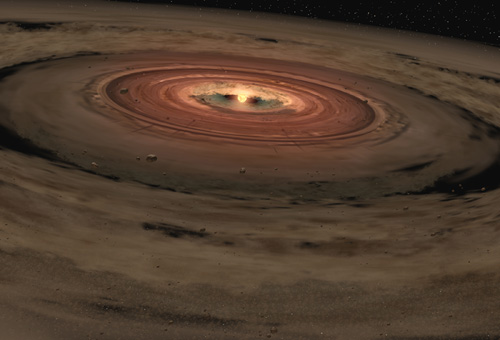
The development of our solar system is probably the closest celestial-scale event which led to us, and as such it offers some of the greatest insights into how we came to be on this not too warm nor too cold planet. From learning of comets and their delivery of ices to the early planets, to the way gas giants like Jupiter protect inner planets from larger objects by changing their course with their immense gravitational pull, the way the solar system, ours especially, has developed in a unique way to arrive at the evolution of life is a source of continual amazement and further investigation. To learn if this happens elsewhere, if there are other corners of the galaxy and beyond which have led to such a delicate, yet resilient and unyielding, system, we continue to build telescopes to search beyond what our eyes can perceive, including the Kepler space telescope and other missions on their way. One thing is certain: understanding how we got here will be a never-ending pursuit, and we wouldn’t want it any other way. 

References: 

Carroll, B. W., & Ostlie, D. A. (2007). The Early Universe. In B. W. Carroll, & D. A. Ostlie, An Introduction to Modern Astrophysics. San Francisco: Pearson: Addison Wesley.

 http://www.daviddarling.info/images/protoplanetary_disk.jpg

Starry Art

We are bounded in a nutshell of Infinite Space: Week 9: Free Form #12: Starry Art

I have, in previous occasions, shown how I have wandered into the intersections of my interests/ hobbies with the study of astronomy. As could be seen from the usual type of post I write which doesn’t include the huge digression of mathematics, I tend to focus on art, history, and mythology, but none of these is nearer to me than art: the pursuit of representing the cross of the human spirit and the world we inhabit. Starting several years ago, I began to develop techniques and proper artistic ability through continuous exploration and reproduction, leading up to now being able to know what I have to improve, and identifying the ways the old masters created their art, in order to learn and apply what they developed to my style. As such, one of the paintings I produced in recent years was titled “Bent Light”:

Rodrgo Cordova, 2014

Here, I developed a piece made entirely with oil paints, based on the effect of a black hole on the perception of the light coming from distant celestial objects. It illustrates how the movement of light in distant galaxies is changed and distorted when a singularity in the fabric of space is put in its way, as is the case of a black hole (for more on lensing: check out http://ay16-rodrigocordova.blogspot.com/2015/09/what-does-microlensing-look-like.html ) The light is the constant, the limit, of the universe, the maximum speed of any object, particle, or wave. The ultimate expression of the maximum movement. This is what I tried to represent: the maximum movement of the universe, meeting with the epitome of the immovable object: a black hole. These two extremes are united in this picture, creating an incredible image in space which has been captured myriad times by telescopes on this Earth and above it. It is through images like this one that the beauty of the universe can be captured, not through elegant equations which rightly explain the universe, but do little to express its majesty. This is also true of how most images received from the telescopes finally arrives in the public eye: artists who interpret data and images with several filters in order to create the mystifying images of space we have seen for the past decades.

The artist’s role in astronomy is no less important than the developers of the telescope or the theorist behind the project, for they are all quintessential in understanding, interpreting, and appreciating the astronomy, harkening back to the first drawings of the Galilean moons and the craters of the Moon. We could not even picture our own Galaxy were it not for the artistic minds and hands which make dreams, imagination, and binary codes, into the illustrations of the world beyond ours.

Rodrgo Cordova, 2016

To Starry Nights

We are bounded in a nutshell of Infinite Space: Week 9: Free Form #11: To Starry Nights

Astronomy could now be the pursuit of astronomers, astrophysicists, men and women of science who attempt to understand the mechanics of stellar movement and the ways the skies change and evolve. This has been true for centuries if not millennia, with figures as old as Galileo Galilei and Hipparchus, each contributing to the understanding of the heavenly spheres. However, there was another group, just as important, who considered the effect the stars and their image had on the imagination of the humans who stared at them every night. These are the artists, the interpreters of the intersection of reality and imagination, the surreal and real, the bit of the human spirit which refuses to yield to the oppressiveness of life and the continuous struggles it contains, all framed by canvas and substances which originated in dying stars eons ago. The clearest example of an artist impassioned by the heavens is Vincent Van Gogh, the creator of Starry Night

and Starry Night Over the Rhone.

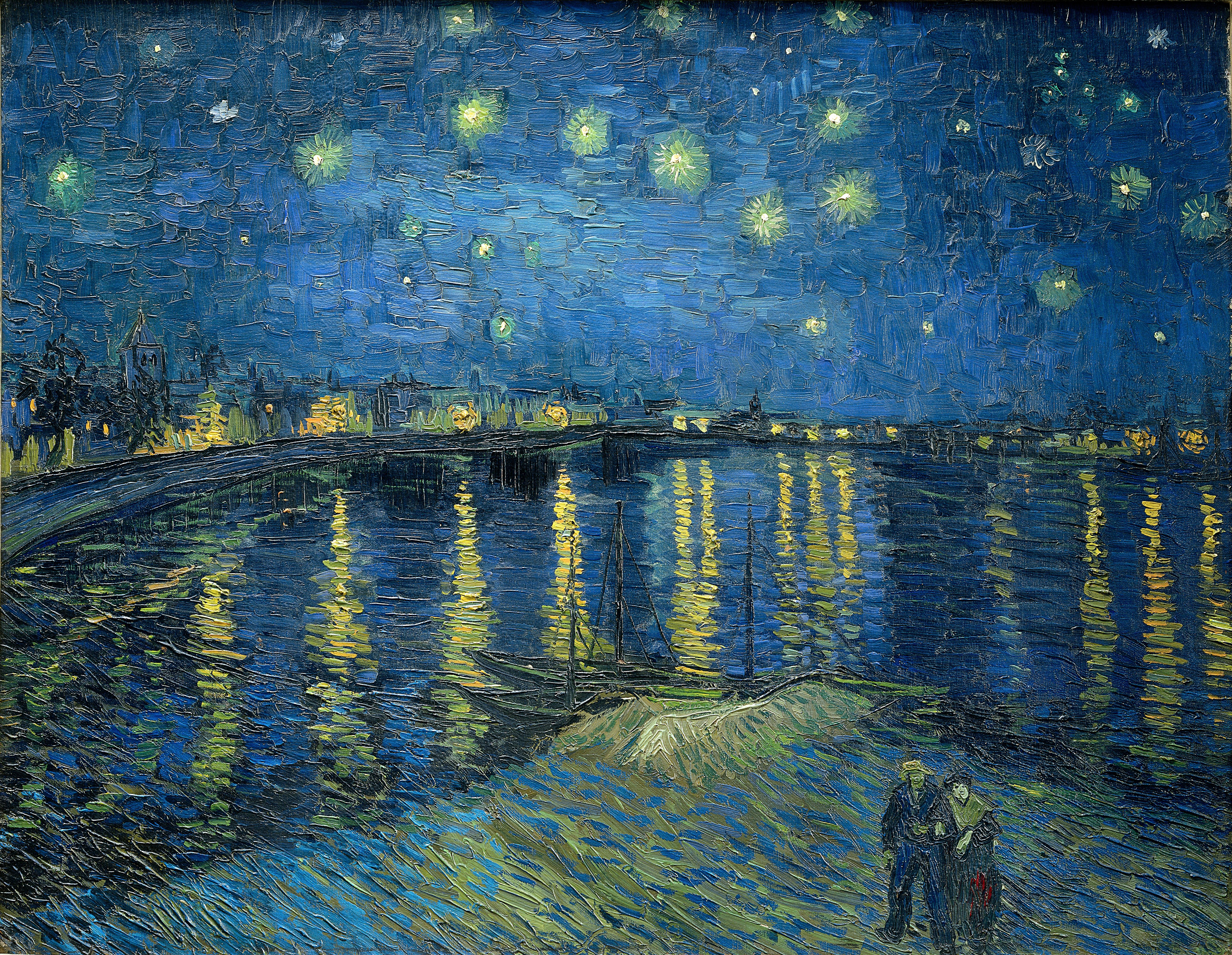
Van Gogh is but one example of how the stars have influenced humanity’s creativity and the development of our culture. Beyond the present conceptions of nuclear reactors, stars were light, sources of divine inspiration as it were, a fundamental part of how humans have developed, looking up at the worlds beyond our understanding, to then attribute myths, tales, origin stories, and a range of ideas all attempting to connect us with the horizon of our imagination.  We spent millennia seeing the stars, wondering whether they were the evidence of our creation, the source of protection (as Van Gogh would paint in Starry Night), or the source of all we know and treasure. Little did we know then that, in fact, all we see around us had its origin 13.68 billion years ago, all from the same place, all form the first stars till the first galaxies to now the dot we reside on. 

References:

http://uploads3.wikiart.org/images/vincent-van-gogh/the-starry-night-1889(1).jpg!Large.jpg

https://upload.wikimedia.org/wikipedia/commons/9/94/Starry_Night_Over_the_Rhone.jpg

Stars from Molecular Clouds

We are bounded in a nutshell of Infinite Space: Week 9: Worksheet #16: Problem #1: Stars from Molecular Clouds   

1. Forming Stars Giant molecular clouds occasionally collapse under their own gravity (their own “weight”) to form stars. This collapse is temporarily held at bay by the internal gas pressure of the cloud, which can be approximated as an ideal gas such that \(P = nkT\), where n is the number density (\(cm^{-3} \)) of gas particles within a cloud of mass M comprising particles of mass \(\bar{m}\) (mostly hydrogen molecules, \(H_2\)), and k is the Boltzmann constant, \(k = 1.4 \times 10^{16} erg K^{-1} .

(a) For a spherical molecular cloud of mass M, temperature T, and radius R, relate the total thermal energy to the binding energy using the Virial Theorem, recalling that you used something similar to kinetic energy to get the thermal energy earlier. (HINT: a particle moving in the \(i^{th}\) direction has \( E_{thermal}  = \frac{1}{2} mv_i^2 = \frac{1}{2} kT\). This fact is a consequence of a useful result called the Equipartition Theorem.)

(b) If the cloud is stable, then the Virial Theorem will hold. What happens when the gravitational binding energy is greater than the thermal (kinetic) energy of the cloud? Describe in words.

(c) What is the critical mass, \(M_J\) , beyond which the cloud collapses? This is known as the “Jeans Mass.” Assume a cloud of constant density \(\rho\).

(d) What is the critical radius, \(R_J\), that the cloud can have before it collapses? This is known as the “Jeans Length.”

(e) The time for a self-gravitating cloud to collapse is often estimated by the “free-fall timescale,” or the time it would take a cloud to collapse to a point in the absence of any resistance. We’ll derive this timescale and use it to re-derive the Jean’s Length. Consider a test particle in an \(e \approx 1\) orbit around a point mass equal to the cloud’s mass. The time it takes for a point mass to move from R to the central mass, or half an orbit, is equivalent to the free-fall timescale. Recall that \(e = 0\) would be a circular orbit, and make sure you can draw what an \(e \approx 1\) orbit looks like. Use \(M = \frac{4}{3} \pi r^3\]  to frame this expression in terms of a single variable—the average density, \(\bar{\rho}\). \[t_{ff} = \sqrt{\frac{3\pi}{ 32G\rho}}\]  

(f) If the free-fall timescale of a cloud is significantly less than a “dynamical timescale”, or the time it takes a pressure wave (sound wave with speed \(c_s\) )to traverse the cloud, the cloud will be unstable to gravitational collapse. Use dimensional analysis to derive the relationship between the sound speed, the cloud’s pressure, P, and the mean density. Then derive the dynamical timescale, the time it takes a pressure wave to cross the cloud of radius R.

(g) Equate the free fall time to the sound crossing time and solve for the maximum R. This maximum is Jeans Length, \(R_J\) , which we derived previously. Use the ideal gas law to ascertain that the two equations for Jeans length matches, at least if we neglect constants of order unity due to assumptions of the system’s geometry.

(h) For simplicity, consider a spherical cloud collapsing isothermally (constant temperature, T) with initial radius \(R_0 = R_J\) . Once the cloud radius reaches \(0.5 R_0\), by what fractional amount has \(R_J\) changed? What might this mean in terms of the number of stars formed within a collapsing molecular cloud? (This is the concept of fragmentation.)

a. From the Virial Theorem, we know that: \[ K = -\frac{1}{2} U,\] which then turns into the thermal energy in the three degrees of freedom for the movement of particles in space, and the potential energy is described by the gravitational potential of a particle: \[ \frac{1}{2} kT +\frac{1}{2} kT+\frac{1}{2} kT = -\frac{1}{2} \frac{-GMm}{R},\]  which simplifies down to \[ 3kT = \frac{GMm}{R},\] the relationship of thermal and gravitational energy.

However, the system should be solved for the entire system of particles, which turns into: \[ 3NkT = \frac{3}{5} \frac{GM^2}{R},\] from the addition of the N particles and a precious derivation we have done to describe the gravitational potential of a system of particles, becoming: \[ 5NkT = \frac{GM^2}{R}.\]

b. Furthermore, if we compare the two sides of the equation, and ask ourselves what would happen if the left side were less than the right: \[ NkT < \frac{1}{5} \frac{GM^2}{R} ,\]  we see that this is actually pressure and gravity, and thus the conclusion of having overpowering gravity becomes clear: \[ P < G,\] the system would collapse.  

c. Now, knowing how the total number of particles is the same as the mass of the enture system over the mass of an individual particle, we see: \[\frac{M_J}{\bar{m}} = N ,\] as well as knowing that the density of a system can be described as: \[ \rho = \frac{M_J}{\frac{4}{3} \pi R_J^3},\] and consequently as \[ R_J = \left(\frac{M_J}{\frac{4}{3} \pi \rho}\right)^{1/3}. \] From these definitions and the understanding of the Jean’s Mass, we can rewrite the above equation from (a):  \[ NkT = \frac{1}{5} \frac{GM_J ^2}{R_J} \] \[ \frac{M_J}{\bar{m}} kT = \frac{1}{5} \frac{GM_J ^2}{\left(\frac{M_J}{\frac{4}{3} \pi \rho}\right)^{1/3}},\] and so we have this turn into:  \[ \frac{5kT}{\bar{m}} = GM_J \times \frac{\left(\frac{4}{3} \pi \rho\right)^{1/3}}{M_J^{1/3}},\] and is continuously simplified till we have: \[ \frac{5kT}{\bar{m}} = GM_J ^{2/3} \left(\frac{4}{3} \pi \rho \right)^{1/3},\] the accurate representation of how we determine the Jean’s Mass: \[M_J = \left(\frac{5kT}{(4\rho)^{1/3} G \bar{m} }\right)^{3/2}\]

d. Next, we find the critical radius at which any greater the molecular cloud would begin to collapse. Starting off from the same principles from the derivation of Jean’s Mass, but now we use the density to solve for \(R_J\) : \[ NkT = \frac{1}{5} \frac{GM_J ^2}{R_J}\] \[N = \frac{M_J}{\bar{m}}\] \[ \frac{M_J}{\bar{m}}kT = \frac{1}{5} \frac{GM_J ^2}{R_J}\] \[ R_J = \frac{1}{5} \frac{GM_J \bar{m}}{kT}\] \[ \rho = \frac{M_J}{\frac{4}{3} \pi R_J^3},\] now we convert the mass into terms of the Jean’s Length: \[ M_J = \rho \cdot \frac{4}{3} \pi R_J^3 ,\] and now have: \[ R_J = \frac{1}{5} \frac{G(\rho \cdot \frac{4}{3} \pi R_J^3)\bar{m}}{kT},\] which becomes: \[ R_J = \left(\frac{15 kT }{ 4 G \rho \pi \bar{m}}\right)^{1/2},\] and can be quickly simplified to reduce the amount of constants till we have: \[ R_J = \left(\frac{5 kT }{ 4 G \rho \bar{m}}\right)^{1/2},\] the correct equation for finding the critical length of a molecular cloud.  

e. Furthermore, we can find the free fall time for which the cloud would collapse: assuming we have an object which practically falls directly to the center once its orbit is of \[ e \approx 1\] (for a problem very similar to this we need at the beginning of the school year, visit http://ay16-rodrigocordova.blogspot.com/2015/09/we-are-bounded-in-nutshell-of-infinite_13.html )

So, the time is precisely, in terms of other orbital systems:  \[t_{ff} = \frac{P}{2},\] which from Kepler’s third law we can rewrite as: \[ t_{ff} = \frac{1}{2} \left(\frac{4\pi^2 a^3}{GM}\right)^{1/2},\] and now simplifying the system we see how:  \[ t_{ff}= \frac{1}{2} \frac{2\pi a^{3/2}}{(GM)^{1/2}}\] \[ t_{ff} = \frac{\pi a^{3/2}}{(GM)^{1/2}}.\] Next, we must describe the mass in terms of the density of the molecular cloud and the distance the free fall is traveling (R).  \[ M = \frac{4}{3} \pi R^3 \rho,\] furthermore, the semi major axis of the orbit then becomes only a portion of the total distance covered, precisely:  \[ a = \frac{R}{2},\] and then all this information is once again placed within our larger equation: \[ t_{ff} = \frac{\pi \left(\frac{R}{2}\right)^{3/2}}{G^{1/2} \cdot \left(\frac{4}{3} \pi R^3 \rho \right)^{1/2}},\] which reduces down to: \[ t_{ff} = \left(\frac{\pi^2 \frac{1}{8}}{G \frac{4}{3} \pi \rho}\right)^{1/2},\] and we thus have the free fall time for the collapse of a molecular cloud: \[ t_{ff} = \left(\frac{3\pi}{32 G \rho}\right)^{1/2},\] identical to what the question asks for.  

f. Now, considering the way information propagates within a molecular cloud, at the speed of “sound” or vibrational energy: we know its dimensions are: \[ c_s \sim \frac{Dist.}{time},\] and we can relate this to other properties of the cloud through dimensional analysis: \[ P \sim \frac{\frac{Mass\cdot Dist.}{time^2}}{Dist.^2}\] \[ P = \frac{M}{t^2 D}\] \[ \rho = \frac{Mass}{Dist.^3}.\] Now that we know these dimensions for pressure and density, there is a way to relate them so they produce a speed. This is by: \[ c_s = \sqrt{\frac{P}{\rho}} ,\]  which we test through dimensional analysis: \[ \frac{D}{t} = \sqrt{\frac{\frac{M}{t^2D}}{\frac{M}{D^3}}} = \sqrt{\frac{D^2}{t^2}},\] therefore: \[c_s \propto \sqrt{\frac{P}{\rho}}.\] And in fact, this is the correct equation for describing the propagation of sound in a pressured medium: \[c_s = \sqrt{\frac{P}{\rho}}.\]

Also, we can use this equation to describe the distances traveled and the relation to the time it takes for the information to travel, which we know from the previous problem comes to:  \[ \frac{R}{c_s} = t_{ff}.\]

g. Therefore, we can use this information of how free fall time and the speed of sound/information propagation to find the Jean’s Length once again. From the previous part, we know: \[ \frac{R_J}{c_s} = t_{ff},\] which becomes as we plug in the full representation of these components: \[ \frac{R_J}{sqrt{\frac{P}{\rho}}} = \left(\frac{3\pi}{32 G \rho}\right)^{1/2},\] and simplifying the equation, we get: \[\frac{R_J^2 \rho}{P} = \frac{3\pi}{32 G \rho}\] \[ R_J^2 = \frac{3\pi P}{32 G \rho^2},\] we also know the other definition of pressure:  \[ P = nkT\] \[ R_J^2 = \frac{3\pi nkT}{32 G \rho^2}\] but we also know, from previous parts, that: \[ n = \frac{\rho}{\bar{m}},\] which is the number density of the system. Taking both of these into account, we turn the equation into:  \[ R_J^2 = \frac{3\pi kT}{32 G \rho \bar{m}},\] which ultimately yields the “same” equation we had for Jean’s Length previously, although some of the constants have changed due to the changes in the assumptions: \[ R_J = \left(\frac{3\pi kT}{32 G \rho \bar{m}} \right)^{1/2}.\]

h. In the beginning of the problem, we have a large molecular cloud of size \(R_0\), which we then learn has decreased to a size \(0.5 R_0\). Therefore, the Jean’s length, which is inherently tied to the initial length because of the factor of the density of the molecular cloud, changes as well. Simplifying the equation for \(R_J\) into the variables we care about, we see how  \[ R_J = \left(\frac{3\pi kT}{32 G \rho \bar{m}} \right)^{1/2},\] becomes \[ R_J \propto \sqrt{\frac{T}{\rho}}.\] However, we also know that the temperature stays constant, and as such the proportion turns into \[ R_J \propto \sqrt{\frac{1}{\rho}}.\] Now we introduce the reduction in the length by a factor of \(\frac{1}{2}\): \[ R_J \propto \sqrt{\frac{1}{R^3}} \] \[ R_J \propto \sqrt{\frac{1}{\frac{1}{2}^3}} \] \[ R_{J_{new}} \propto \sqrt{8} \] and so the proportion of the change is: \[\frac{R_{J_{old}}}{ R_{J_{new}}} = \frac{1}{\sqrt{8}}= \frac{1}{2\sqrt{2}}\] Therefore, the fraction of the molecular cloud that is the Jean’s length now is smaller than the decrease in the overall molecular cloud length (\(\frac{1}{2} R_0\). This means the size of the molecular cloud is larger than the Jean’s Length, setting of fragmentation. This process describes how a molecular cloud fragments and begins collapsing within itself in clouds the size of the Jean’s Length, internal to the overall cloud. This process continues as the collapse spawns several smaller clouds, which each begin collapsing within themselves, following a fractal pattern of collapse. They continue on this trend until they are small and dense enough to become stars, the endgame of Molecular Clouds. 

Electron at its finest

We are bounded in a nutshell of Infinite Space: Week 9: Worksheet #15: Problem #1: Electron at its finest 

1. Hydrogen Ionization: The interstellar medium is ionized by UV photons from stars. The goal of this worksheet is to explore the ionization process and how it regulates much of the observed structure of the ISM close to massive stars, and the diffuse ISM everywhere.

(a) Hydrogen energy levels: Outside of molecular clouds, the most abundant species in the ISM is atomic hydrogen (in molecular clouds it is molecular hydrogen). Whether the ISM is fully ionized or not will therefore depend on how easily atomic hydrogen is ionized. The ground electronic state of a hydrogen atom corresponds to an atom with the smallest (and hence most tightly bound) electron orbit around the nuclear proton that is consistent with a stationary electronic wave function, a standing wave. The electronic energy levels permitted by quantum mechanics are characterized by their quantum numbers n=1 2 3, where n=1 corresponds to the ground state. Make a drawing of the electronic energy levels of atomic hydrogen. Mark out the energy needed to excite an atom in its ground state to a free proton and electron. Illustrate what happens in case of photoionization.

(b) Ionizing stars: Remember that stars are blackbodies. Which kind of stars emit a majority of their photons with energies high enough to photo ionize (excite an electron into freedom) ground state hydrogen. Give your answer in both stellar surface temperature, and letter classification.

(c) Excitation state of hydrogen: But why do we only care about excitation from the ground state to free protons and electrons? After all if hydrogen is in an excited state (e.g. n=2) you could use many more of the available stellar photons to ionize the ISM. The lifetime of an excited state is \(\sim 10^{-9} s\). Let’s calculate the time scale of ionization right next to the star to test whether it is reasonable to assume that all hydrogen are in their ground state. First, set up an equation for the ionization rate for a single hydrogen atom in terms of the photon flux and the ionization cross section \(\sigma\). The ionization cross section is \(10^{-17} cm^2\) . Calculate the photon flux assuming that you are sitting right next to the star from (b) and that the star is emitting all its energy in the form of photons with the exact energy required to ionize atomic hydrogen.

How do the two time scales compare? Is it reasonable to assume that all hydrogen is in the ground state?

(d) Recombination: The inverse of photoionization is recombination. In a recombination event an electron and proton collide and become bound while emitting a photon. Illustrate a recombination event. Set up an equation for the recombination rate in terms of the number densities of protons, electrons and the rate coefficient \(\alpha\), which describes the efficiency at which a recombination occurs when an electron and proton collides. Note that a recombination can happen to any hydrogen energy level (n=1,2,3 etc). If the recombination takes the hydrogen immediately to the ground state you will produce a new ionizing photon. If the recombination take the hydrogen into any other level the emitted photon will not be able to ionize another hydrogen atom.

a.

b. Starting from the basic equations we have learned for blackbodies, we use Wein’s Law: \[ \lambda_{peak} = \frac{0.3 cm\cdot K}{ T}\] and the equation describing the energy of a photon: \[ E = h\nu\] and the relationship of wavelength and frequency: \[ c = \lambda \nu\] \[\nu = \frac{c}{\lambda},\] and now we can retroactively plug in the equations to describe how a specific photon energy is emitted by a star at a specific temperature: \[E = \frac{hc}{\lambda}\] \[ \lambda = \frac{hc}{E},\] \[ \frac{hc}{E} = \frac{0.3 cm\cdot K}{ T}\] \[T = \frac{0.3cm\cdot K \cdot E }{hc},\] Now that we have placed the equation in terms of the temperature, we can place the constants, including Planck’s Constant in eV, and values for energy of ionization:  \[ T = \frac{0.3cm\cdot K \cdot (13.6 eV) }{\left(3\times 10^{10} \frac{cm}{s} \right)(4.14 \times 10^{-15} eV \cdot s)},\]  This solves to the temperature at which stars will produce energy sufficient to cause the ionization of hydrogen. \[T = 3.29 \times 10^4 K \to ~ an~O/B~ star\] 

c. Next, we will use the temperature we have just found to describe the Ionization rate the star creates. Knowing the base equation for the rate: \[ I = j \sigma,\] we solve for the photon flux by first determining the flux at the surface of the star:  \[F = \sigma T^4 ,\]  and plugging the value for the temperature we had just found and the Stephan Boltzmann Constant: \[ T = \left(5.7 \times 10^{-5} \frac{1}{K^4} \right)( 3.3 \times 10^4 K )^4 ,\] which yields: \[ F = 6.75 \times 10^{13} \frac{ergs}{cm^2 s}.\] However, we now have to convert this into photon flux, meaning we apply dimensional analysis and find that: \[ F = 6.75 \times 10^{13} \frac{ergs}{cm^2 s} \times \frac{1 eV}{ 1.6 \times 10^{-12} ergs} \times \frac{1 ~photon}{13.6 eV},\] which in turn tells us the photon flux  \[ j = 3.1 \times 10^{24} \frac{photons}{cm^2 s},\] now going back to the original equation, we see that: \[I = j\sigma,\] and just plugging in the constant given in the problem and the value we just derived: \[I =  \left(3.1 \times 10^{24} \frac{photons}{cm^2 s}\right) (10^{-17} cm^2),\] the ionization rate is thus: \[ I = 3.1 \times 10^7 \frac{photons}{s}.\] Next we have to understand the timescale for atoms to get ionized: \[\frac{1}{I} = Timescale,\] such that: \[Timescale = \frac{1}{3.1 \times 10^7 \frac{photons}{s}} = 3.2 \times 10^{-8} \frac{s}{photon}\] Therefore, the timescale is 30 times that of the excited state duration, meaning the decay is much quicker than the time necessary to ionize the atom.

d. Recombination is when a proton and electron combine to form a stable atom once again after being ionized, which occurs at a rate of \[ Volumetric ~Recombination ~Rate = \frac{\# ~Recombinations}{t \cdot Volume},\] which is directly proportional to the density of protons and electrons found in the volume:  \[r_v \propto n_e n_p \] \[r_v = \alpha n_e n_p\]

As seen in the illustration above, the collision produces excess energy which is represented by \[  E_\gamma = E_{tot} - 13.6 eV, \] in the case of collision which produced another ionizing photon.