The universe is REALLY old and REALLY big

We are bounded in a nutshell of Infinite space: Blog Post #27, Worksheet # 8.1, Problem #3: The universe is REALLY old and REALLY big

3. It is not strictly correct to associate this ubiquitous distance-dependent redshift we observe with the velocity of the galaxies (at very large separations, Hubble’s Law gives ‘velocities’ that exceeds the speed of light and becomes poorly defined). What we have measured is the cosmological redshift, which is actually due to the overall expansion of the universe itself. This phenomenon is dubbed the Hubble Flow, and it is due to space itself being stretched in an expanding universe.

Since everything seems to be getting away from us, you might be tempted to imagine we are located at the center of this expansion. But, as you explored in the opening thought experiment, in actuality, everything is rushing away from everything else, everywhere in the universe, in the same way. So, an alien astronomer observing the motion of galaxies in its locality would arrive at the same conclusions we do.

In cosmology, the scale factor,\(a(t)\)  is a dimensionless parameter that characterizes the size of the universe and the amount of space in between grid points in the universe at time t. In the current epoch, \( t = t_0\)  and \(a(t_0) \equiv 1\)  . \(a(t)\)  is a function of time. It changes over time, and it was smaller in the past (since the universe is expanding). This means that two galaxies in the Hubble Flow separated by distance \(d_0 = d(t_0) \) in the present were \(d(t) = a(t) d_0 \)   apart at time t.

The Hubble Constant is also a function of time, and is defined so as to characterize the fractional rate of change of the scale factor:

\[H(t) = \frac{1}{a(t)} \frac{da}{dt}|_t\] and the Hubble Law is locally valid for any t: \[ v = H(t)d\] where v is the relative recessional velocity between two points and d the distance that separates them.

(a) Assume the rate of expansion, \(\dot{a} = da/dt \), has been constant for all time. How long ago was the Big Bang (i.e. when \(a(t=0) = 0\) )? How does this compare with the age of the oldest globular clusters\(\sim 12 Gyr)? What you will calculate is known as the Hubble Time.

(b) What is the size of the observable universe? What you will calculate is known as the Hubble Length.

(a) In this problem, we’ll be examining some of the first methods developed that correctly estimated the age, and size of the universe (from our perspective). Going back to one of the pioneers in the field of cosmology, Edwin Hubble established a set of relationships and constants which have largely determined the basis for all cosmology. One of these basics is the Hubble constants, a value found by analyzing the Red Shifts of many galaxies and comparing them all in their velocities and distance from Earth. The slope of this graphical comparison yields the Hubble Constant, which can be approximated to being \( 70 \frac{\frac{km}{s}}{Mpc} \). Knowing this, we can start to use calculus and integrate the above calculation for the Hubble Constant as a function of time when \(a(t) = a(t_0)\): \[H(t_0) = \frac{1}{a(t_0)} \frac{da}{dt}|_{t=0} , \] \[H(t_0) = \frac{da}{dt} , \] \[ dt = \frac{da}{ H(t) } , \] and now we integrate to find the total \(H(t)\) : \[\int_{t=0}^{t=present} dt = \int^{a(t_0)}_0 \frac{da}{ H(t) } , \] \[t = H_0 ^{-1} .\] And now, plugging in the compiled value for Hubble Time, we can convert it to an actual time by making the dimensional analysis work. So if \( H_0 = 70 \frac{\frac{km}{s}}{Mpc} , \) then we simply find the value of km in pc, and turn Mpc into pc, so the final dimensional analysis would be: \[ H_0 = 70 \frac{\frac{km}{s}}{Mpc} \cdot ( 3.24 \times 10^{-20} \frac{pc}{s} ) \cdot (1 \times 10^{-6} \frac{Mpc}{pc} ) ,\] which yields: \[H_0 = 2.27 \times 10^{-18} \frac{1}{s} ,\]  and once this is plugged into the equation for the age of the universe we found a just a bit ago, we now have: \[t = \frac{1}{2.27 \times 10^{-18}  s^{-1}} ,\] \[ t = 4.41 \times 10^{17} s\] and now we just convert this value into years so it looks like it makes sense: \[ t =  4.41 \times 10^{17} s \cdot (3600 \frac{s}{hour}) \cdot (24 \frac{hours}{day}) \cdot (365 \frac{days}{year}) ,\] \[t = 1.4 \times 10^{10} years ,\] a close approximation to the current definition for the age of the universe, which is 200 million years older than the oldest globular cluster we have observed.

(b) To find the Total Distance of the galaxy, it is as simple as multylping the age of the universe times the maximum speed of the universe, the speed of light. So by taking the speed of light and turning it into the distance it travels in one year: \[ c = 3 \times 10^8 \frac{m}{s} \cdot (3600 \frac{s}{hour}) \ cdot (24 \frac{hours}{day}) \cdot (365 \frac{days}{year}) , \] \[c = 9.46 \times 10^{15} \frac{m}{year} , \] and next we turn the speed of light into Mpc per year: \[ c = 9.46 \times 10^{15} \frac{m}{year} \cdot \frac{1}{3.241 \times 10^23 \frac{m}{Mpc} } , \] \[c = 2.77 \times 10^{-8} \frac{Mpc}{year} , \] and now finally multiply this by the age of the universe and we get: \[1.4 \times 10^{years} ~years ~\cdot 2.77 \times 10^{-8} \frac{Mpc}{year} = 3.87 \times 10^2 Mpc .\] However, this is not the total observable distance of the universe, rather it is only the radius of our line of sight, so to complete the distance, we would need to multiply this radius by 2 to get the total diameter of the sphere that we consider the observable universe, the Hubble Length. \[ Hubble ~Length= 2 \times  3.87 \times 10^2 Mpc ,\] \[Hubble ~Length = 7.7 \times 10^2 Mpc . \]

Introduction to growth in infinite directions

We are bounded in a nutshell of Infinite space: Blog Post #26, Worksheet # 8.1, Problem #1: Introduction to growth in infinite directions

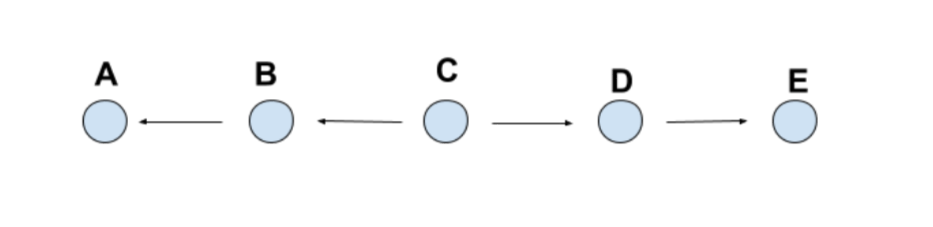
1. Before we dive into the Hubble Flow, let’s do a thought experiment. Pretend that there is an infinitely long series of balls sitting in a row. Imagine that during a time interval \(\Delta t\) the space between each ball increases by \(\Delta x\).

(a) Look at the shaded ball, Ball C, in the figure above. Imagine that Ball C is sitting still (so we are in the reference frame of Ball C). What is the distance to Ball D after time \(\Delta t\)? What about Ball B?

(b) What are the distances from Ball C to Ball A and Ball E?

(c) Write a general expression for the distance to a ball N balls away from Ball C after time \(\Delta t\). Interpret your finding.

(d) Write the velocity of a ball N balls away from Ball C during \(\Delta t\). Interpret your finding.

(a) As Edwin Hubble trained his telescope onto the greater heavens, objects thousands if not hundreds of thousands of light years away, he began to see the hints of something in play in the universe, something few had ever thought of conceiving as possible. Since ancient times, the Earth was the center of the cosmos, with everything rotating around it, an idea disproven during the Scientific Revolution. But even these great minds did not envision how humanity would later understand how there were galaxies and clusters and unimaginably large structures in the cosmos which left Hubble with a clear idea: the universe was growing, every second, of every day. The expansion Hubble saw can be described by various methods, mainly by his own Hubble Constant, but more on that in the next post.

First let us discuss how this expansion works, how objects that are spaced from each other all move at a same speed, but because of their original place, they continually look farther and farther away.

In the example of a row of balls, we have the question of how much distance separates B and D from C, in its point of view. For each case, the distance to B or D is \(\Delta x\), as is established by the question after a time \(\Delta t\).

(b) The same reasoning applies to balls A and E, where if the space from B to A has to be \(\Delta x\) and if the distance from C to B is already \(\Delta x\), then the distance from C to A has to be \(2 \Delta x\), a case identical to ball E.

(c) So, if the balls’ position away from the point of reference is the guiding force driving the distance it has after a time \(\Delta t\), a ball N balls away will always be \(N \Delta x\) away after a time \(\Delta t\). So the equation for the distance from the ball C will always be: \[D(\Delta t) = N\Delta x .\] This shows, and we’ll get more into this in just a bit, that the farther an object was at the start, the farther it will move after a time \(\Delta t\)

(d) Now that we have a general equation for the distance from the point of reference, we can use it to find the velocity of the object for any original condition. From kinematics we already know the equation for distance traveled by an object with constant velocity is: \[X_f = X_i + v(\Delta t) ,\] which can be rewritten as: \[ v = \frac{X_f – X_i }{\Delta t} ,\] \[ v = \frac{\Delta x}{\Delta t}, \] which happens to be very similar to the equation for distance we have already found. Now we simply plug in the actual distance equation for the case of a constant expansion as we have been describing: \[v = \frac{N \Delta x}{\Delta t}, \] which describes the velocity of an object we are viewing from a particular reference point. From it, we can clearly see that an object that is farther away is perceived to be moving increasingly faster, a fact which has helped astronomers many times.

As we will see in the next post, apparent and actual velocities help a great deal, permitting us to understand just how far away an object is (giving us a new rung on the distance ladder to use as necessary), as well as how long its light has been traveling, but more on this next time.

Gas, gas everywhere and every-when

We are bounded in a nutshell of Infinite space: Blog Post #25, Worksheet # 7.2, Problem #5: Gas, gas everywhere and every-when

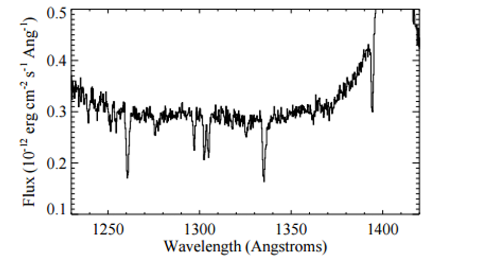
5. You may also have noticed some weak “dips” (or absorption features) in the spectrum:

(a) Suggest some plausible origins for these features. By way of inspiration, you may want to consider what might occur if the bright light from this quasar’s accretion disk encounters some gaseous material on its way to Earth. That gaseous material will definitely contain hydrogen, and those hydrogen atoms will probably have electrons occupying the lowest allowed energy state.

(b) A spectrum of a different quasar is shown below. Assuming the strongest emission line you see here is due to \(L\gamma\alpha\), what is the approximate red-shift of this object?

(c) What is the most noticeable difference between this spectrum and the spectrum of 3C 273? What conclusion might we draw regarding the incidence of gas in the early Universe as compared to the nearby Universe?

(a) These features could be caused by the way the elements found in the gas of the interstellar medium have the ability, like all atoms, to absorb energy and thus dim the light we receive from the original source. However, if we take these absorption numbers, we can then find the exact composition of the interstellar gas, since only specific wavelengths can be absorbed and used within the internal mechanics of the atom.

(b) As to the Red Shift of this new emission spectrum, the process is almost identical to the process made for problem #4. Knowing the Red Shift Equation, we have:   \[\frac{\lambda_{observed} - \lambda_{emitted}}{\lambda_{emitted}}  = z ,\] which is just a matter of plugging in the emitted wavelength of hydrogen, since the peak of this spectrum is the hydrogen emission (as the problem establishes), which is 1215.67 \(\dot{A}\). The Other value would be the wavelength of the max flux, which is 5625 Angstroms. So the equation is: 
\[\frac{5625 \dot{A}  - 1215.67 \dot{A}}{1215.67 \dot{A}}  = z,  \] \[ z =3.627, \] which is the Red Shift of this emission spectrum.

(c) Considering both the emission spectrum we just analyzed and the spectrum for 3C 273, the one we studied previously, there seems to be a major difference. The emission is shifted for the fact of the Red Shift as a result of the quasar being farther away, therefore faster from our perspective, and thus older. But the clear distinction is how the 3C 273 graph had much fewer dips during the beginning of the spectra, while the new quasar is absolutely full of dips before it rises to the max Flux. This helps to show that this galaxy, being farther away and older than other stars, hints at how the universe was long ago: full of gas, unformed and ready to be turned into the next generations of stars and planets.

Quantum mechanics and Black Hole Mass, all wrapped up in a nice problem

We are bounded in a nutshell of Infinite space: Blog Post #24, Worksheet # 7.2, Problem #3 & #4: Quantum mechanics and Black Hole Mass, all wrapped up in a nice problem.  

3 & 4. Such bright objects, known as quasars, can be easily observed at great distances, and astronomers started taking spectra of them back in the 1960’s. Here’s a spectrum of the first quasar ever discovered, called 3C 273:

What are the main features you see in this spectrum (ignoring the gap in the data at around 1625 \(\dot{A}\)?

One feature you surely noticed was the strong, broad emission lines. Here is a closer look at the strongest emission line in the spectrum:

This feature arises from hydrogen gas in the accretion disk. The photons radiated during the accretion process are constantly ionizing nearby hydrogen atoms. So there are many free protons and electrons in the disk. When one of these protons comes close enough to an electron, they recombine into a new hydrogen atom, and the electron will lose energy until it reaches the lowest allowed energy state, labeled n = 1 in the model of the hydrogen atom shown below (and called the ground state):

On its way to the ground state, the electron passes through other allowed energy states (called excited states). Technically speaking, atoms have an infinite number of allowed energy states, but electrons spend most of their time occupying those of lowest energies, and so only the n = 2 and n = 3 excited states are shown above for simplicity. Because the difference in energy between, e.g., the n = 2 and n = 1 states are always the same, the electron always loses the same amount of energy when it passes between them. Thus, the photon it emits during this process will always have the same wavelength. For the hydrogen atom, the energy difference between the n = 2 and n = 1 energy levels is 10.19 eV, corresponding to a photon wavelength of \(\lambda\) = 1215.67 Angstroms. This is the most commonly-observed atomic transition in all of astronomy, as hydrogen is by far the most abundant element in the Universe. It is referred to as the Lyman α transition (or Lyα for short). It turns out that that strongest emission feature you observed in the quasar spectrum above arises from \(l \gamma \alpha\)  emission from material orbiting around the central black hole.

(a) Recall the Doppler equation: \[\frac{\lambda_{observed} - \lambda_{emitted}}{\lambda_{emitted}}  = z ≈ \frac{v}{c}\] Using the data provided, calculate the redshift of this quasar.

(b) Again using the data provided, along with the Virial Theorem, estimate the mass of the black hole in this quasar. It will help to know that the typical accretion disk around a \(10^8 M_\odot\) black hole extends to a radius of \( r = 10^{15} m.\)

(a) As we can see from the graphs, a main characteristic of the emission spectra is the high peak, which we interpret as the main light output from Hydrogen atoms changing energy levels, one of the most common, if not the most common, occurrences in the universe. Knowing this is hydrogen, we can compare its emission spectra to that of what we know it should be from experiments on Earth, and some great conclusions can be drawn from this experiment.

Understanding the nature of how light propagates is essential to this problem. Here, an object, namely another galaxy, is moving away from the Milky Way, understood as evidence of the expanding universe, since all galaxies are continually moving outwards and expanding the space they occupy as a whole. Furthermore, this expansion is incredibly fast, going at speeds comparable to the speed of light, which offers astronomers the opportunity to better understand how galaxies move and how far away they are. This method is easy enough to understand, using the equation for a Doppler Shift, as you might have learned from a physics class (for sound waves and their wavelengths) we can use the same one to compare what we know the wavelengths of light should be and compare it with the observed wavelength. So we take:  \[\frac{\lambda_{observed} - \lambda_{emitted}}{\lambda_{emitted}}  = z ,\] where z is the Red Shift (the analog of Doppler Shift for light). Knowing Hydrogen’s emission peaks at 1215.67 Angstroms ( \(10^{-10} m \) ) and from the zoomed in graph we know the peak of this emission spectra is around 1406 Angstroms. These can be plugged into the equation and we get: \[\frac{1406 \dot{A} - 1215.67 \dot{A} }{1215.67\dot{A}}  = z ,\] and thus the red shift of this galaxy is: \[z = .1566 ,\] which can be used to approximate the speed of the galaxy as well and, consequently, understand the time its light has taken to reach us.

(b) From previous problems, we know the virial theorem is an equation which permits us to use a simple relationship between the kinetic and potential energies in a galaxy. (See full Virial Theorem explanation in http://ay17-rcordova.blogspot.com/2015/10/energy-in-space-is-anything-but-one.html ). Furthermore, by taking the Virial Theorem and expanding it with the full definition of Flux, Luminosity, and Potential Energy, we get an equation which describes a relationship between Luminosity and the mass of the black hole which creates the accretion disk. The full equation is as follows: \[L = \frac{G M_{SMBH} \cdot 4\pi\cdot c\cdot M_{Proton}}{\sigma_t},\] where G is the gravitational constant, c is the speed of light, and \(\sigma_t\) is the Thomson Cross Section, valued at \(6.6524 \times 10^{-25} cm^2 \), which is the effective area of an electron interacting with a photon. This equation can be rewritten to fit the data given in the problem, Flux. BY dividing both sides by \(4\pi r^2\) we have: \[\frac{L}{4\pi r^2}= \frac{G M_{SMBH}\cdot c\cdot M_{Proton}}{r^2 \sigma_t},\] \[F_{SMBH}= \frac{G M_{SMBH}\cdot c\cdot M_{Proton}}{r^2 \sigma_t}.\] Taking this into account, and knowing the value of the mass of a proton is \(1.6726219 \times 10^{-24} g , \) as well as the problem establishing that the radius of the black hole is  \( r = 10^{15} m\). Plugging in all the values we have accumulated, and solving for the mass of the Black Hole, we have: \[F_{SMBH}= \frac{G M_{SMBH}\cdot c\cdot M_{Proton}}{r^2 \sigma_t},\]  \[\frac{F_{SMBH} \cdot r^2 \cdot \sigma_t }{G \cdot c \cdot M_{Proton} }=  M_{SMBH}, \]  \[  M_{SMBH}= \frac{\left(0.93 \times 10^{12} \frac{erg}{cm^2 s}\right) \cdot (10^{17} cm)^2 \cdot (6.6524 \times 10^{-25} cm^2) }{(6.67 \times 10^{-8} \frac{cm^3}{g~s^2})\cdot (3 \times 10^{10}\frac{cm}{s} )\cdot (1.6726219 \times 10^{-24} g) } , \]   \[  M_{SMBH}= 1.85 \times 10^42 g , \] and this is the mass of the black hole we have been studying. 

Why we explore space.

We are bounded in a nutshell of Infinite space: Blog Post #23, Free Form #4: Why we explore space.

        In most cases, this blog attempts to convey the how, the means by which the amazing phenomena which are peered at through huge lenses occur and how they unfold, how they are described and understood. I could now do the same thing, speak to how the human race has risen from its humblest beginnings, looking at the stars above and seeing themselves in them, as we rightly should. I could describe how we, puny specks on a pale blue dot, managed to develop amazing technologies which enabled us to go to the moon, to reach the fourth planet from our star, to send a man-made object outside our own solar system, but few would listen. The how has become boring, part of the so-called “rocket science” so many revere, disapprove of, or believe themselves incapable of understanding. Our society has forgotten why we explore space, why we search for the complete unknown, why we are willing to invest in people who work on projects which will not bear fruit for decades, why sacrificing funding for new projects sometimes, rarely in the modern age, was better than ignoring and defunding the work scientists have done for the past century.

       So now, in the most recent election cycle, the United States, like most democratic nations, chooses its leaders after months of parades, speeches, shows, hyperboles and spectacles, where to speak about space is to speak of immediate poll drops. The facts are these, the National Aeronautics and Space Administration (NASA) of the United States has become a third rail of politics, not the agency which defined the modern world. Its funding, from among the largest sixty years ago, has now been reduced to less than a percent of the U.S. Federal Budget, and every day more and more scientists are unable to pursue the research they want for lack of funding, or the difficulty in procuring it. Another fact, the once acme of all science and scientific discovery, the U.S.; the place where the atom was split, where men were sent to land on the moon, where polio was cured, and where the greatest amount of Nobel Laureates in a single country live, is ranked 27^th in Mathematics, 20^th in Science, and 17^th in Reading. Although these numbers are clearly marked by the steep social disparity in the United States, the fact remains the best graduates of the public schooling system in the United States are still years behind the best students graduating from the systems in China, Hong Kong, Korea, and Japan, among others. Nevertheless, this is a solvable problem, it is an attainable change, but to do so, it will require an event, a sudden change which will leave the entire world reeling, a cataclysmic or miraculous incident that will redefine humanity… like it’s happened before. 

      In the last 100 years, there have been two World Wars, a Cold War, and the scientific accomplishments just mentioned. Every single one of these events triggered...something. The Second World War spurred the creation of the Polio vaccine, the Cold War prompted a nation not 200 years old to plan to go to the moon within a decade of setting this course, and the creation of a scientific tool inspired millions to use it to spread messages, ideas, radical statements, and revolutions, at the speed of fiber-optic cables across this world wide web. Furthermore, when the words a “giant leap for mankind” thundered throughout the world, it dawned the modern age of science and research, it inspired millions to go out and learn, to lead new fields, and usher in the next age of humanity.

     So what happened? What changed in the perspectives of society so science was no longer the goal of humanity? This was once the trend, long ago when science was thought to be the practice of alchemists, and it has become this once again. The modern age has seen a resurfacing of the same idea that science is a discipline to be thought of as occult teachings, knowledge to be feared, and in the minds of some revered. But this does not even include the main reason science is our greatest tool, the fact of it being fallible, disprovable, human.

      Therefore, a new “small step for [a] man” is necessary, a demonstration of human innovation and a reiteration of our potential, and there are few who are capable delivering on a promise such as this. The fact remains, we’ve done it before, and there are enough of us willing to make it happen once again. Beyond the technological marvels created in the endeavor to reach the next interstellar destination, the effect new discoveries have on the world; beyond the possibility of new materials and sheer brain-power concentrated on tasks which only benefit humanity. Why we explore space awakens something deeper. Space is the next step, it is as the New World was to the 15^th century, and it is what will continue to harken to our sense of exploration. We are inspired to reach for the stars, to then look beyond them, while remembering the fragile blue sphere and recognize it as our home, one we are charged with caring for. We are all humans, product of 13.68 billion years of stellar evolution… and as innate as a child searching for its parents, we must understand where we came from and who we are, for it is part of our being.

References: 
http://www.businessinsider.com/pisa-rankings-2013-12
http://www.oecd.org/unitedstates/PISA-2012-results-US.pdf
http://www.nasa.gov/mission_pages/apollo/apollo11.html
http://i.imgur.com/2wNay.jpg

All the light you can barely see

We are bounded in a nutshell of Infinite space: Blog Post #22, Worksheet # 7.1, Problem #6: All the light you can barely see


6. If your telescope can detect optical magnitudes \(m_V \leq 21\) how far away, in parsecs, can you detect a Type Ia supernova with your telescope? (HINT: The Sun’s absolute magnitude is \(M_V =4.83\) .)


Here, we’ll be going back to some of our earlier problems involving distance moduli and Luminosity and magnitude comparisons. From previous problems and known astronomical facts, we have:


\[L_{Ia} = 3.1308 \times 10^{43} \frac{ergs}{s} ,\] the luminosity of the sun is: \[L_\odot = 3.846 \times 10^{33} \frac{ergs}{s} ,\] and the equation for comparing absolute magnitudes is \[M_\star - M_\odot = -10^{0.4} \log_10 \left(\frac{L_\star}{L_\odot}\right) . \] Having these values, as well as the Absolute Magnitude of the sun, given by the problem, \(M_V =4.83\), then we can simply solve for the absolute magnitude of the Supernova. \[M_{Ia} - M_\odot = -10^{0.4} \log_{10} \left(\frac{L_{Ia}}{L_\odot}\right) ,\] \[M_{Ia}= -10^{0.4} \log_{10} \left(\frac{L_{Ia}}{L_\odot}\right) + M_\odot,\] \[M_{Ia}= -10^{0.4} \log_{10} \left(\frac{3.1308 \times 10^{43} \frac{ergs}{s}}{3.846 \times 10^{33} \frac{ergs}{s}}\right) + 4.83,\] \[ M_{Ia}= -24.8944 + 4.83,\] \[M_{Ia} = -20.061.\]


Now knowing the absolute magnitude of the supernova, we can now solve for the maximum distance when the max apparent magnitude that can be recorded is 21. Using \[m – M = 5 \log_{10} (d) -5 ,\] \[ d \leq 10^{\frac{m- M  +5}{5}} ,\] \[ d\leq 10^{\frac{21- (-20.06)  +5}{5}} ,\] \[ d\leq 10^{9.212} ,\] \[ d \leq 1.629 \times 10^ 9 pc = 1.629 \times 10^6 kpc ,\] which is the max distance our telescopes can see with present technology, for now.

What E= mc^2 actually does

We are bounded in a nutshell of Infinite space: Blog Post #21, Worksheet # 7.1, Problem #5: What \(E= mc^2 \) actually does

5. Gamma rays from the radioactive decay of nickel into iron drive most of the optical luminosity of a Type-Ia supernova. The process is given by: \[^{56}Ni \to ~ ^{56}Co + \gamma \to ~ ^{56}Fe + \gamma \] , where \(\gamma\) represents photons. 

The atomic weights of \(^{56} Ni\) and \(^{56} Fe\) are 55.942135 and 55.934941 amu, respectively. Let’s calculate the total energy radiated in the optical wavelengths during the event, given that the characteristic times for the two decay processes are 8.8 days and 111 days, respectively.

(a) Let’s balance the decay process from \(^{56} Ni\) to \(^{56} Fe\) for a single atom, ignoring the intermediate step. According to the first law of thermodynamics, energy cannot be created or destroyed. Use the fact that \(E= mc^2 \) to balance the equation.

(b) How many nickel atoms are there in the white dwarf? Use this number to estimate the total energy emitted in photons.

(c) Now combine the characteristic times for the two processes to find a total characteristic time. Divide the energy you found in part (b) by this time scale to find a characteristic luminosity.

(a) For this problem, a bit of chemistry could be necessary, but more important than that, its understanding the nature of what we are describing. A White Dwarf is a star that has been compressed and become composed of mostly heavy materials, such as nickel, iron, and other, heavier atoms. Because of the density, a White Dwarf, although small, is incredibly massive, and can thus release enormous amounts of energy in spectacular fashions. White dwarfs are also important because they are believed to be the star that initiates a type Ia Supernova explosion, a major part of the cosmic distance ladder we have explored in previous posts.

Now, we’ll see just how luminous these explosions are, which is when a White Dwarf starts initiating a reaction ending in a dazzling flash that outshines the galaxy it inhabits. This process begins, as the problem describes, with \[^{56}Ni \to ~ ^{56}Co + \gamma \to ~ ^{56}Fe + \gamma , \] a chemical process which releases the mass of the atoms in the form of pure energy, as photons. So as Nickel turns into Cobalt and then into Iron, the difference in the mass between the last and first step is: \[M(^{56}Ni) - M(^{56}Fe) = 55.942135 amu - 55.934941 amu , \] \[M(^{56}Ni) - M(^{56}Fe) = 0.007194 amu , \] where amu is atomic mass unit, and this mass represents the mass of the atoms turned into pure energy in the form of part of the electromagnetic spectrum in photons.

Taking this number and changing it into a cgs standard measurement, we use the mass of a proton per amu and multiply it by the change in mass: \[M_{Proton} = 1.6726219 \times 10^{-24} \frac{g}{amu} , \] \[\Delta M \cdot M_{Proton} = 0.007194 amu \cdot 1.6726219 \times 10^{-24} \frac{g}{amu} ,\] \[\Delta M \cdot M_{Proton} = .012032842 \times 10^{-24} g  ~.\]

Now we use the famous equation, \(E= mc^2 \), and plug in the value of the mass changed into energy per atom and constant of the universe, c, the speed of light. \[E = mc^2 , \] \[E_{Photon} = .012032842 \times 10^{-24} g   \cdot \left(3 \times 10^{10} \frac{cm}{s} \right)^2 ,\] \[E_{Photon}  = 1.083 \times 10^{-5} ergs . \]

(b) From earlier problems, we know the maximum mass a White Dwarf can have is \( M_{WD} = 1.4 M_\odot \) and if we were to divide this total mass by the mass of a single atom of 56 Nickel, we would find the total amount of Nickel atoms in a White Dwarf. So, knowing the mass of the sun is: \[M_\odot = 2 \times 10^{33} g ,\] \[ M_{WD} = 1.4 \times \times  2 \times 10^{33} g ,\] \[ M_{WD} = 2.8 \times 10^{33} g.\] And now finding the mass of an atom of nickel in grams as we found the mass turned  into photons: \[ M(^{56}Ni )= 55.942135 amu,\] \[M_{Proton} = 1.6726219 \times 10^{-24} \frac{g}{amu} , \] \[ M(^{56}Ni) = 55.942135 amu \times 1.6726219 \times 10^{-24} \frac{g}{amu} , \] \[ M(^{56}Ni )= 9.35700040134 \times 10^{-23}  g/atom .\] And now we divide the total mass of the star by the mass of an atom: \[\frac{M_{WD}}{ M(^{56}Ni )} = \frac {2.8 \times 10^{33} g }{9.35700040134 \times 10^{-23}  g/atom} \] \[^{56} +Ni~atoms~in~a~WD = 2.9424 \times 10^{55} atoms .\]

Since we have already found the energy produced by a single atom of 56 Nickel, we can take this photon energy, multiply it by the amount of atoms, and understand the energy the White Dwarf releases: \[Energy~Emitted= ~^{56}Ni~atoms~in~a~WD \cdot E_{Photon}  ,\] \[ Energy~Emitted = 2.9424 \times 10^{55} atoms \cdot 1.083 \times 10^{-5} \frac{ergs}{atom} ,\] \[ Energy~Emitted = 3.2406 \times 10^{50} ergs .\]

(c) Now that we know the energy that is produced in total by the explosion of the White Dwarf in photons, we can use this to find its Luminosity, a measure of energy over time. From the problem, we know the time period for the entire atomic process to occur is 8.8 days + 111 days, a total of 119.8 days. And turning this timescale into seconds, we have: \[ 119.8 days \times 24 \frac{hours}{day} \times 60 \frac{min}{hour} \times 60 \frac{seconds}{min} = 10,350,720 ~seconds\] Take these two values, and dividing them, we have the characteristic luminosity of the White Dwarf/Supernova Explosion: \[L = \frac{Energy~Emitted}{Period} ,\] \[L = \frac{3.2406 \times 10^{50} ergs }{1.0350720 \times 10^7 s},\] \[L= 3.1308 \times 10^{43} \frac{ergs}{s} .\]

One Theory for how White Dwarfs become Ia Supernovae

And another one

References:

https://astrofauna.files.wordpress.com/2012/04/merger_animation_rd255.gif

http://hetdex.org/images/dark_energy/supernova_explosion_34452.jpg